Combinations of transformations

← Back: Homogeneous coordinates

Overview: Transformations

Next: Inverse transformation →

In the previous subarticle homogeneous coordinates and transformation matrices for translation and rotation around the three axes are introduced:

$\mathbf{Trans}(p_x,p_y,p_z), \quad\mathbf{Rot}(x,\varphi), \quad \mathbf{Rot}(y,\varphi), \quad\mathbf{Rot}(z,\varphi)$

These transformation matrices can be combined by multiplying them.

Consider the following transformation matrix $\mathbf{T}$ that corresponds to the multiplication of several single transformation matrices (also denoted with $\mathbf{T}$ for simplification):

$\mathbf{T}=\mathbf{T}_n...\mathbf{T}_3\mathbf{T}_2\mathbf{T}_1$

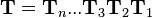
Combinations of transformations are always applied from right to left. So in the example case, $\mathbf{T}_1$ is applied first. Then on this result, transformation $\mathbf{T}_2$ is applied and so on. The left transformation matrix $\mathbf{T}_n$ is finally multiplied with the result of all the previous transformations.

As already stated for multiplication of matrices, different multiplication orders lead to different results. If only translations are regarded, the order does not matter, because translation is actually vector addition and vector addition is commutative. Rotation however depends on the current input coordinates. Descriptively seen, rotation is always applied around the origin or around an axis intersecting with the origin, respectively. So the rotational part is depending on the respective current coordinates. Different orders of transformations result in different input coordinates for each transformation.

The following example shows descriptively as well as computationally, that the order of transformations is important (see figure on the right). Consider a local coordinate frame positioned in the origin, whose axes are oriented parallel to the global coordinate axes. The related initial position vector $\vec{\mathbf{q}}_0$ is a zero vector. A translation matrix 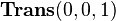$\mathbf{Trans}(0,0,1)$ and a rotation matrix $\mathbf{Rot}(x,90^\circ)$ are to be applied to this local frame. So two different orders of the two transformations are possible.

The upper three subfigures on the right show the first case. The local frame is first rotated around the x-axis and then translated on the z-axis. The result is shown in the top right subfigure. Computationally $\vec{\mathbf{q}}_0$ is first pre-multiplied with $\mathbf{Rot}(x,90^\circ)$ and then pre-multiplied with $\mathbf{Trans}(0,0,1)$:

$\begin{align} \vec{\mathbf{q}}_1&= \left[\begin{array}{c} x_1\\ y_1\\ z_1\\ 1 \end{array}\right]= \mathbf{Trans}(0,0,1)\mathbf{Rot}(x,90^\circ)\vec{\mathbf{q}}_0 = \left[\begin{array}{cccc} 1 & 0 & 0 & 0\\ 0 & 1 & 0 & 0\\ 0 & 0 & 1 & 1\\ 0 & 0 & 0 & 1 \end{array}\right] \left[\begin{array}{cccc} 1 & 0 & 0 & 0\\ 0 & 0 & -1 & 0\\ 0 & 1 & 0 & 0\\ 0 & 0 & 0 & 1 \end{array}\right] \left[\begin{array}{c} x_0\\ y_0\\ z_0\\ 1 \end{array}\right] \\ &= \left[\begin{array}{cccc} 1 & 0 & 0 & 0\\ 0 & 0 & -1 & 0\\ 0 & 1 & 0 & 1\\ 0 & 0 & 0 & 1 \end{array}\right] \left[\begin{array}{c} x_0\\ y_0\\ z_0\\ 1 \end{array}\right]= \left[\begin{array}{c} x_0\\ -z_0\\ y_0+1\\ 1 \end{array}\right]= \left[\begin{array}{c} 0\\ 0\\ 1\\ 1 \end{array}\right] \end{align}$

The lower three subfigures on the right show the second case. The local frame is first translated on the z-axis and then rotated around the x-axis. The result is shown in the lower right subfigure. Computationally $\vec{\mathbf{q}}_0$ is first pre-multiplied with $\mathbf{Trans}(0,0,1)$ and then pre-multiplied with $\mathbf{Rot}(x,90^\circ)$:

$\begin{align} \vec{\mathbf{q}}_2&= \left[\begin{array}{c} x_2\\ y_2\\ z_2\\ 1 \end{array}\right]= \mathbf{Rot}(x,90^\circ)\mathbf{Trans}(0,0,1)\vec{\mathbf{q}}_0 = \left[\begin{array}{cccc} 1 & 0 & 0 & 0\\ 0 & 0 & -1 & 0\\ 0 & 1 & 0 & 0\\ 0 & 0 & 0 & 1 \end{array}\right] \left[\begin{array}{cccc} 1 & 0 & 0 & 0\\ 0 & 1 & 0 & 0\\ 0 & 0 & 1 & 1\\ 0 & 0 & 0 & 1 \end{array}\right] \left[\begin{array}{c} x_0\\ y_0\\ z_0\\ 1 \end{array}\right] \\ &= \left[\begin{array}{cccc} 1 & 0 & 0 & 0\\ 0 & 0 & -1 & -1\\ 0 & 1 & 0 & 0\\ 0 & 0 & 0 & 1 \end{array}\right] \left[\begin{array}{c} x_0\\ y_0\\ z_0\\ 1 \end{array}\right]= \left[\begin{array}{c} x_0\\ -z_0-1\\ y_0\\ 1 \end{array}\right]= \left[\begin{array}{c} 0\\ -1\\ 0\\ 1 \end{array}\right] \end{align}$

the general homogeneous transformation matrix $\mathbf{T}$ were introduced. $\mathbf{T}$ consists of a rotation matrix and a translation vector:

$\mathbf{T}= \left[\begin{array}{ccc|c} & & & \\ & \mathbf{R} & & \vec{\mathbf{p}}\\ & & & \\ \hline 0 & 0 & 0 & 1 \end{array}\right]$

As shown in the subarticle homogeneous coordinates, multiplication of $\mathbf{T}$ with a vector corresponds to rotating the coordinates first and then adding the translation vector.

Pre-/Post-...

transformation matrices for translation and rotation around the three axes are introduced:

$\mathbf{Trans}(p_x,p_y,p_z), \quad\mathbf{Rot}(x,\varphi), \quad \mathbf{Rot}(y,\varphi), \quad\mathbf{Rot}(z,\varphi)$