Rotation

← Back: Translation

Overview: Transformations

Next: Homogeneous coordinates →

Rotation is a transformation where the coordinates are rotated around the origin of the global coordinate system. The direction of the rotation is defined by the rotation axis, about which the rotation is applied. To determine the direction, the right-hand-rule shown in the figure on the left can be used. If the thumb is pointing in the direction of the rotation axis, the other fingers indicate the rotation direction for positive angles.

In this article rotation is first described for two dimensions and based on the two-dimensional transform matrix, rotation in three-dimensional space is presented.

Two-dimensional

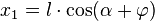
The figure on the right shows an example, where the vector $\vec{\mathbf{q}}_0$ is rotated by $\varphi$ around the origin, what results in vector $\vec{\mathbf{q}}_1$. The rotation axis in this case is pointing out of the figure in the direction of the imaginary $z$-axis. The length of the vector $\vec{\mathbf{q}}_0$ is assumed as $l$ and so the length of $\vec{\mathbf{q}}_1$ is $l$ as well. The initial angle of $\vec{\mathbf{q}}_0$ relative to the x-axis is $\alpha$. Hence the resulting coordinates $x_1$ and $y_1$ can be computed as follows:

$x_1=l\cdot\cos(\alpha+\varphi)$

$y_1=l\cdot\sin(\alpha+\varphi)$

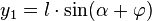
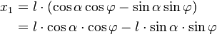
Using the addition theorems of sine and cosine leads to:

$\begin{align} x_1&=l\cdot(\cos\alpha\cos\varphi-\sin\alpha\sin\varphi) \\ &=l\cdot\cos\alpha\cdot\cos\varphi-l\cdot\sin\alpha\cdot\sin\varphi \end{align}$

$\begin{align} y_1&=l\cdot(\sin\alpha\cos\varphi-\cos\alpha\sin\varphi) \\ &=l\cdot\sin\alpha\cdot\cos\varphi-l\cdot\cos\alpha\cdot\sin\varphi \end{align}$

Regarding the vector $\vec{\mathbf{q}}_0$ and its angle $\alpha$ to the x-axis, $x_0$ equals $l\cos\alpha$ and $y_0$ equals $l\sin\alpha$. By applying this the above equations can be reformed to:

$x_1=x_0\cos\varphi-y_0\sin\varphi$

$y_1=y_0\cos\varphi+x_0\sin\varphi$

These two equations for $x_1$ and $y_1$ can also be written in matrix notation:

$\left[\begin{array}{c} x_1\\ y_1 \end{array}\right] = \left[\begin{array}{cc} \cos\varphi & -\sin\varphi\\ \sin\varphi & \cos\varphi \end{array}\right] \cdot \left[\begin{array}{c} x_0\\ y_0 \end{array}\right] = \left[\begin{array}{cc} x_0\cos\varphi-y_0\sin\varphi\\ x_0\sin\varphi+y_0\cos\varphi \end{array}\right]$

So the transformation matrix for rotation about $\varphi$ in two dimensions is:

$\mathbf{R}(\varphi) = \left[\begin{array}{cc} \cos\varphi & -\sin\varphi\\ \sin\varphi & \cos\varphi \end{array}\right]$

Example: rotation in two-dimensional space The rotation of a rectangle corresponds to the rotation of each of the three position vectors of the corners individually. The red rectangle is the initial one. If it is rotated by 30 degrees, the result is the blue rectangle. The corresponding transformation matrix is: ${\mathbf{R}}^{r\rightarrow b} = \left[\begin{array}{cc} \cos (30^\circ) & -\sin (30^\circ)\\ \sin (30^\circ) & \cos (30^\circ) \end{array}\right] = \left[\begin{array}{cc} \frac{\sqrt{3}}{2} & -0.5\\ 0.5 & \frac{\sqrt{3}}{2} \end{array}\right]$ The green rectangle is obtained by rotating the red rectangle by 90 degrees. This corresponds to the following transformation matrix: ${\mathbf{R}}^{r\rightarrow g} = \left[\begin{array}{cc} \cos (90^\circ) & -\sin (90^\circ)\\ \sin (90^\circ) & \cos (90^\circ) \end{array}\right] = \left[\begin{array}{cc} 0 & -1\\ 1 & 0 \end{array}\right]$ Another possibility to obtain the green rectangle is rotating the blue rectangle by 60 degrees. Then the transformation matrix is: ${\mathbf{R}}^{b\rightarrow g} = \left[\begin{array}{cc} \cos (60^\circ) & -\sin (60^\circ)\\ \sin (60^\circ) & \cos (60^\circ) \end{array}\right] = \left[\begin{array}{cc} 0.5 & -\frac{\sqrt{3}}{2}\\ \frac{\sqrt{3}}{2} & 0.5 \end{array}\right]$ The back transformation of the blue rectangle to the red rectangle for example is done by the following transformation matrix: ${\mathbf{R}}^{b\rightarrow r} = \left[\begin{array}{cc} \cos (-30^\circ) & -\sin (-30^\circ)\\ \sin (-30^\circ) & \cos (-30^\circ) \end{array}\right] = \left[\begin{array}{cc} \frac{\sqrt{3}}{2} & 0.5\\ -0.5 & \frac{\sqrt{3}}{2} \end{array}\right]$

Three-dimensional

In three-dimensional space three basic types of rotation are regarded: rotation around x-, y- and z-axis. These three types are defined by the axis and the rotation angle $\varphi$ and denoted as $\mathbf{Rot}(x,\varphi)$, $\mathbf{Rot}(y,\varphi)$ and $\mathbf{Rot}(z,\varphi)$.

Rotation around one one of the three coordinate axes changes two components of the coordinates while the component on the rotation axis stays as it is. Hence the properties of two-dimensional rotation can also be used for three-dimensional rotation. The rotation matrix for rotation around the z-axis for example equals the identity matrix with the two-dimensional rotation matrix $\mathbf{R}$ replacing the four top left components:

$\mathbf{Rot}(z,\varphi)= \left[\begin{array}{ccc} \mathbf{\cos\varphi} & \mathbf{-\sin\varphi} & 0\\ \mathbf{\sin\varphi} & \mathbf{\cos\varphi} & 0\\ 0 & 0 & 1 \end{array}\right]$

As the coordinates are rotated around the z-axis, the x- and y-components are calculated as in two-dimensional space (see above) and the z-component stays as it is:

$\left[\begin{array}{c} x_1\\ y_1\\ z_1 \end{array}\right]= \left[\begin{array}{ccc} \mathbf{\cos\varphi} & \mathbf{-\sin\varphi} & 0\\ \mathbf{\sin\varphi} & \mathbf{\cos\varphi} & 0\\ 0 & 0 & 1 \end{array}\right] \cdot \left[\begin{array}{c} x_0\\ y_0\\ z_0 \end{array}\right]= \left[\begin{array}{c} x_0\cos\varphi-y_0\sin\varphi\\ x_0\sin\varphi+y_0\cos\varphi\\ z_0 \end{array}\right]$

Accordingly the rotation matrices for the x- and y-axis are:

$\mathbf{Rot}(x,\varphi)= \left[\begin{array}{ccc} 1 & 0 & 0\\ 0 & \cos\varphi & -\sin\varphi\\ 0 & \sin\varphi & \cos\varphi \end{array}\right]$

$\mathbf{Rot}(y,\varphi)= \left[\begin{array}{ccc} \cos\varphi & 0 & \sin\varphi\\ 0 & 1 & 0\\ -\sin\varphi & 0 & \cos\varphi \end{array}\right]$

The three colums of the rotation matrix describe the new coordinate axes. The first colum corresponds to the new x-axis, the second column to the new y-axis and the third to the new z-axis:

$\mathbf{Rot}= \left[\begin{array}{ccc} \vec{\mathbf{x}}_n & \vec{\mathbf{y}}_n & \vec{\mathbf{z}}_n\\ \end{array}\right]$

Example: Three-dimensional rotation The figure on the right shows a colored coordinate frame in the black global coordinate system. The left subfigure shows the initial situation, the initial position vector $\vec{\mathbf{q}}_0$ and three colored axes are the following: $\vec{\mathbf{q}}_0= \left[\begin{array}{c} 0\\1\\0 \end{array}\right] ,\qquad \vec{\mathbf{x}}_0= \left[\begin{array}{c} 1\\0\\0 \end{array}\right] ,\qquad \vec{\mathbf{y}}_0= \left[\begin{array}{c} 0\\1\\0 \end{array}\right] ,\qquad \vec{\mathbf{z}}_0= \left[\begin{array}{c} 0\\0\\1 \end{array}\right]$ The colored coordinate frame is then rotated around the x-axis by 90 degrees. The corresponding rotation matrix is: $\mathbf{Rot}(x,90^\circ)= \left[\begin{array}{ccc} 1 & 0 & 0\\ 0 & \cos90^\circ & -\sin90^\circ\\ 0 & \sin90^\circ & \cos90^\circ \end{array}\right] = \left[\begin{array}{ccc} 1 & 0 & 0\\ 0 & 0 & -1\\ 0 & 1 & 0 \end{array}\right]= \left[\begin{array}{ccc} \vec{\mathbf{x}}_1 & \vec{\mathbf{y}}_1 & \vec{\mathbf{z}}_1\\ \end{array}\right]$ The resulting position vector $\vec{\mathbf{q}}_1$ is: $\vec{\mathbf{q}}_1= \mathbf{Rot}(x,90^\circ)\cdot\vec{\mathbf{q}}_0= \left[\begin{array}{ccc} 1 & 0 & 0\\ 0 & 0 & -1\\ 0 & 1 & 0 \end{array}\right]\cdot \left[\begin{array}{c} 0\\1\\0 \end{array}\right] = \left[\begin{array}{c} 0\\0\\1 \end{array}\right]$ As can be seen in the right subfigure the rotation matrix describes the three resulting axes of the colored coordinate frame after the rotation: $\vec{\mathbf{x}}_1= \left[\begin{array}{c} 1\\0\\0 \end{array}\right] ,\qquad \vec{\mathbf{y}}_1= \left[\begin{array}{c} 0\\0\\1 \end{array}\right], \qquad \vec{\mathbf{z}}_1= \left[\begin{array}{c} 0\\-1\\0 \end{array}\right]$