Multiplication of matrices

Overview: Matrices

There are exercises as selftest for this article.

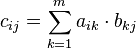
Two matrices can be multiplied if the number of colums of the left matrix equals the number of rows of the right matrix. The result of the multiplication of an l-by-m matrix $\mathbf{A}=(a_{ij})_{i=1...l,j=1...m}$ with an m-by-n matrix $\mathbf{B}=(b_{ij})_{i=1...m,j=1...n}$ is an l-by-n matrix $\mathbf{C}=(c_{ij})_{i=1...l,j=1...n}$ . To calculate the components of the resulting matrix, the components of one row of the first matrix are multiplied with the components of one column of the second matrix respectively and summed up. For example for the component $c_{ij}$ the components of row $i$ of the first matrix are multiplied with the components of column $j$ of the second matrix. This leads to the following equation for the components of $\mathbf{C}$ :

c_{ij}=\sum^{m}_{k=1}a_{ik}\cdot b_{kj}

A clear possibility to compute the resulting matrix is the pattern of Falk. Thereto the first matrix $\mathbf{A}$ is noted and on the right over it the second matrix $\mathbf{B}$ . Then the row vectors of $\mathbf{A}$ and the column vectors of $\mathbf{B}$ lead to l times n intersections which correspond to the l-by-n result matrix $\mathbf{C}$ . The l times n components are determined by computing the dot product of the crossing row vector of $\mathbf{A}$ and column vector of $\mathbf{B}$ :

For example the multiplication of a 2-by-3 matrix with a 3-by-2 matrix results in a 2-by-2 matrix and is computed as follows:

\mathbf{A}\cdot\mathbf{B}= \left[\begin{array}{ccc} a_{11} & a_{12} & a_{13} \\ a_{21} & a_{22} & a_{23} \end{array}\right]\cdot \left[\begin{array}{cc} b_{11} & b_{12} \\ b_{21} & b_{22}\\ b_{31} & b_{32} \end{array}\right]= \left[\begin{array}{cc} a_{11}\cdot b_{11}+a_{12}\cdot b_{21}+a_{13}\cdot b_{31} & a_{11}\cdot b_{12}+a_{12}\cdot b_{22}+a_{13}\cdot b_{12} \\ a_{21}\cdot b_{11}+a_{22}\cdot b_{21}+a_{23}\cdot b_{31} & a_{21}\cdot b_{12}+a_{22}\cdot b_{22}+a_{23}\cdot b_{12} \end{array}\right]

As it holds that 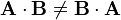$\mathbf{A}\cdot\mathbf{B}\ne\mathbf{B}\cdot\mathbf{A}$ , the order of a matrix product is important. To specify the order, two types of multiplication are distinguished, pre- and post-multiplication. Pre-multiplying a matrix $\mathbf{A}$ by matrix $\mathbf{B}$ means, that $\mathbf{B}$ is written on the left side of the matrix product: $\mathbf{B}\mathbf{A}$ . If matrix $\mathbf{A}$ is post-multiplied by matrix $\mathbf{B}$ , $\mathbf{B}$ is written on the right side: $\mathbf{A}\mathbf{B}$ .

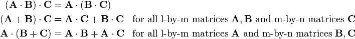
Some further rules for matrix multiplications are:

\begin{align} (\mathbf{A}\cdot\mathbf{B})\cdot\mathbf{C}&=\mathbf{A}\cdot(\mathbf{B}\cdot\mathbf{C}) \\ (\mathbf{A}+\mathbf{B})\cdot\mathbf{C}&=\mathbf{A}\cdot\mathbf{C}+\mathbf{B}\cdot\mathbf{C} &\text{for all l-by-m matrices } \mathbf{A},\mathbf{B} \text{ and m-by-n matrices } \mathbf{C}\\ \mathbf{A}\cdot(\mathbf{B}+\mathbf{C})&=\mathbf{A}\cdot\mathbf{B}+\mathbf{A}\cdot\mathbf{C} &\text{for all l-by-m matrices } \mathbf{A} \text{ and m-by-n matrices }\mathbf{B},\mathbf{C} \end{align}

Example: Multiplication of matrices

A good example for the multiplication of several matrices in the context of robotics and transformations is presented in the robotics script. Please have a look in chapter 3 on page 3-35

Multiplication of matrices with vectors

A vector is a just special form of a matrix with either only one row or one column. Because an l-by-m matrix can only be multiplied by an m-by-n matrix, there are two possibilities of multiplying matrices and vectors. The first possibility is a 1-by-m row vector multiplied with an m-by-n matrix which results in a 1-by-n row vector:

\left[\begin{array}{ccc} v_{11} & \dots & v_{1m} \end{array}\right] \cdot \left[\begin{array}{ccc} a_{11} & \dots & a_{1n}\\ \vdots & \ddots & \vdots\\ a_{m1} & \dots & a_{mn} \end{array}\right] = \left[\begin{array}{ccc} v_{11}a_{11}+\dots+v_{1m}a_{m1} & \dots & v_{11}a_{1n}+\dots+v_{1m}a_{mn} \end{array}\right]

The second possibility is a l-by-m matrix multiplied with an m-by-1 column vector which results in a l-by-1 column vector:

\left[\begin{array}{ccc} a_{11} & \dots & a_{1m}\\ \vdots & \ddots & \vdots\\ a_{l1} & \dots & a_{lm} \end{array}\right] \cdot \left[\begin{array}{c} v_{11}\\ \vdots \\ v_{m1} \end{array}\right] = \left[\begin{array}{c} a_{11}v_{11}+\dots+a_{1m}v_{m1}\\ \vdots \\ a_{l1}v_{11}+\dots+a_{lm}v_{m1} \end{array}\right]

Example: Multiplication of matrices and vectors

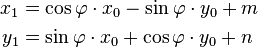
In chapter 3 of the robotics script some examples of matrices multiplied with vectors appear. On page 3-28 a two-dimensional transformation equation is presented for a rotation about $\varphi$ about the origin (see figure) in combination with a translation. The equation uses homogeneous coordinates. The resulting vector is the following: