Inverse transformation

← Back: Combinations of transformations

Overview: Transformations

Next: Three-Angle Representations →

Let $\mathbf{T}$ be a general homogeneous transformation matrix. The inverse transformation $\mathbf{T}^{-1}$ corresponds to the transformation that reverts the rotation and translation effected by $\mathbf{T}$. If a vector is pre-multiplied by $\mathbf{T}$ and subsequently pre-multiplied by $\mathbf{T}^{-1}$, this results in the original coordinates because $\mathbf{T}^{-1}\mathbf{T}=\mathbf{I}$ and multiplication with the identity matrix does not change anything (see transformations).

The general homogeneous transformation matrix $\mathbf{T}$ for three-dimensional space consists of a 3-by-3 rotation matrix $\mathbf{R}$ and a 3-by-1 translation vector $\vec{\mathbf{p}}$ combined with the last row of the identity matrix:

$\mathbf{T}= \left[\begin{array}{ccc|c} & & & \\ & \mathbf{R} & & \vec{\mathbf{p}}\\ & & & \\ \hline 0 & 0 & 0 & 1 \end{array}\right]$

As stated in the article about homogeneous coordinates, multiplication with $\mathbf{T}$ is equivalent in cartesian coordinates to applying the rotation matrix $\mathbf{R}$ first and then translating the coordinates by $\vec{\mathbf{p}}$:

$\vec{\mathbf{q}}_1= \mathbf{T} \cdot \vec{\mathbf{q}}_0 \equiv \mathbf{R}\cdot \vec{\mathbf{q}}_0 + \vec{\mathbf{p}}$

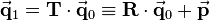
The equation above is now solved for $\vec{\mathbf{q}}_1$. Here the fact is used, that the inverse of 3-by-3 rotation matrices equals the transpose of the matrix:

$\begin{align} \vec{\mathbf{q}}_1&=\mathbf{R} \vec{\mathbf{q}}_0 + \vec{\mathbf{p}} & & \\ \vec{\mathbf{q}}_1-\vec{\mathbf{p}}&=\mathbf{R} \vec{\mathbf{q}}_0 & & \\ \mathbf{R}^{-1}(\vec{\mathbf{q}}_1-\vec{\mathbf{p}})&=\mathbf{R}^{-1}\mathbf{R} \vec{\mathbf{q}}_0 & & \\ \mathbf{R}^{T}(\vec{\mathbf{q}}_1-\vec{\mathbf{p}})&=\mathbf{R}^{T}\mathbf{R} \vec{\mathbf{q}}_0 & & \\ \mathbf{R}^{T}\vec{\mathbf{q}}_1-\mathbf{R}^{T}\vec{\mathbf{p}}&=\vec{\mathbf{q}}_0 \qquad\quad \rightarrow \qquad\quad \vec{\mathbf{q}}_0=&\underbrace{\mathbf{R}^{T}}&\vec{\mathbf{q}}_1+(\underbrace{-\mathbf{R}^{T}\vec{\mathbf{p}}})\\ & &\mathbf{R}_i& \qquad\qquad \vec{\mathbf{p}}_i\\ \end{align}$

Based upon this the inverse of a homogeneous transformation matrix is defined as:

$\mathbf{T}^{-1}= \left[\begin{array}{ccc|c} & & & \\ & \mathbf{R} & & \vec{\mathbf{p}}\\ & & & \\ \hline 0 & 0 & 0 & 1 \end{array}\right]^{-1}= \left[\begin{array}{ccc|c} & & & \\ & \mathbf{R}_i & & \vec{\mathbf{p}}_i\\ & & & \\ \hline 0 & 0 & 0 & 1 \end{array}\right]= \left[\begin{array}{ccc|c} & & & \\ & \mathbf{R}^T & & -\mathbf{R}^T\vec{\mathbf{p}}\\ & & & \\ \hline 0 & 0 & 0 & 1 \end{array}\right]$

So instead of using the Adjugate Formula or the Gauß-Jordan-Algorithm to invert a homogeneous transformation matrix, the integrated rotation matrix $\mathbf{R}$ has just to be transposed. The transpose is then used for the rotational part of the inverse transformation matrix and its negated product with the translation vector corresponds to the translational part. The following example will give a proof for this definition.

Example: Inverse homogeneous transformation Consider the transformation matrix $^R\mathbf{T}_N$ that is introduced in the script on page 3-61 and already used as example for matrix inversion: $^R\mathbf{T}_N = \left[\begin{array}{ccc|c} & & & \\ & \mathbf{R} & & \vec{\mathbf{p}}\\ & & & \\ \hline 0 & 0 & 0 & 1 \end{array}\right]= \left[\begin{array}{cccc} 0 & 1 & 0 & 2a\\ 0 & 0 & -1 & 0\\ -1 & 0 & 0 & 0\\ 0 & 0 & 0 & 1 \end{array}\right] \quad\rightarrow\quad \mathbf{R}=\left[\begin{array}{ccc} 0 & 1 & 0 \\ 0 & 0 & -1\\ -1 & 0 & 0\\ \end{array}\right], \quad \vec{\mathbf{p}}=\left[\begin{array}{c} 2a\\ 0\\ 0 \end{array}\right]$ Now the definition from above is used to compute the inverse transformation: $\begin{align} \mathbf{R}^T&= \left[\begin{array}{ccc} 0 & 0 & -1 \\ 1 & 0 & 0\\ 0 & -1 & 0\\ \end{array}\right] \quad\rightarrow\quad -\mathbf{R}^T\vec{\mathbf{p}}= -\left[\begin{array}{ccc} 0 & 0 & -1 \\ 1 & 0 & 0\\ 0 & -1 & 0\\ \end{array}\right] \left[\begin{array}{c} 2a\\ 0\\ 0 \end{array}\right]= -\left[\begin{array}{c} 0\\ 2a\\ 0 \end{array}\right] = \left[\begin{array}{c} 0\\ -2a\\ 0 \end{array}\right]\\ ^R\mathbf{T}_N^{-1} &= \left[\begin{array}{ccc|c} & & & \\ & \mathbf{R}^T & & -\mathbf{R}^T\vec{\mathbf{p}}\\ & & & \\ \hline 0 & 0 & 0 & 1 \end{array}\right]= \left[\begin{array}{cccc} 0 & 0 & -1 & 0\\ 1 & 0 & 0 & -2a\\ 0 & -1 & 0 & 0\\ 0 & 0 & 0 & 1 \end{array}\right] \end{align}$ In the main article about matrix inversion, exactly this inverse matrix $^R\mathbf{T}_N^{-1}$ has already been prooven to be the correct inverse of $^R\mathbf{T}_N$.