Vector algebra
| ← Back: Table of contents | Overview: Vector algebra | Next: Unit vectors → |
|
|
This article gives a brief explanation of vectors and vector algebra.
A scalar value is just a numeric value. In contrast thereto, a vectorial value has a direction. Examples for vectors are all forces and the velocity, which is directed to the driving direction. Vectors are usually denoted with an arrow, for example  . A three-dimensional vector for example is
![\vec{\mathbf{a}}=
\left[\begin{array}{c}
a_x\\
a_y\\
a_z
\end{array}\right]](/wiki/robotics/images/math/5/8/6/586cf758e989f051f45ebd35c220cc75.png)
where  ,
,  and
and  describe the components of the vector in x-, y- and z-direction. Vectors can be denoted as column and row vectors which is based on matrix algebra. is a so called column vector because the three components are denoted in a column. If you transpose a matrix or a vector, respectively, all the components are mirrored at the first diagonal. So if you define
  as the transposed of column vector you get the corresponding row vector
![\vec{\mathbf{b}}=\vec{\mathbf{a}}^T=
\left[\begin{array}{ccc}
a_x & a_y & a_z
\end{array}\right]](/wiki/robotics/images/math/6/9/f/69f1cf9a008d23bfc850077007beb158.png)
For graphical representations arrows are used that show the direction of the vector and whose length equals its magnitude. The magnitude of a vector is defined as

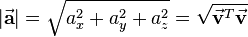
where the last square root contains a standard matrix multiplication.
As the presented notation is comparatively sophisticated  is often reduced to
  . The vector
  has the same magnitude as but is directed opposite. Two or more vectors are called equal if they have the same direction and the same magnitude. The zero vector
  is a special vector with undefined direction and magnitude zero.
Depending on their properties vectors can be characterized as follows:
- Free vector: Free vectors can be moved arbitrarily in space. They are not constrained to a fixed point. So similar vectors can be aligned using translation.
- Constrained vector: Constrained vectors can not be moved because they are constrained to a fixed point in space. A force for example forces act in a certain point and in a certain direction.
- Position vector: Position vectors usually start in the origin of a given coordinate system and point at a certain position of a point. In this sense they are constrained vectors. An example is the position vector of a robot relative to the global coordinate system that is often located in the robots startpoint.
The following subarticles describe the unit vector and the basic arithmetic operations including dot and cross product:
To check whether you are familiar with the presented contents you can test yourself using the provided selftests.
Consider a robot at time
|
 . The robot not only has a current velocity
  but also a direction of motion. Thus the velocity of the robot is a vector
  . The corresponding distance the robot drives then arises out of the product of the velocity vector and the time:
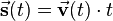
Literature
- Manfred Albach, Grundlagen der Elektrotechnik 1: Erfahrungssätze, Bauelemente, Gleichstromschaltungen, 3. Edition (Pearson Studium, 2011)