Dot product
| ← Back: Simple arithmetic operations | Overview: Vector algebra | Next: Cross product → |
|
|

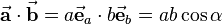
The dot product of two vectors results in a scalar value and is defined as
where  describes the angle between the two vectors which ranges from
  to
to  (see figure). The dot product is denoted with a simple point between the vectors or without any sign.
Regarding the right side of the above equation, the following correlation can be noted: If you project the vector  on the vector
  , you get the distance
  . As a consequence the result of the dot product can be seen as the area of a rectangle with the side legths
  and . The projection can also be done contrariwise (projection of vector on vector ). So that you get the distance
  . The multiplication of this term with
  leads to a rectangle with equivalent area but different aspect ratio (see figure).
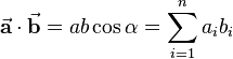
Another possibility to compute the dot product is to multiply the corresponding components and sum them up:

In general the dot product of n-dimensional vectors is computed as follows:
which is nothing else than the matrix product of the transpose of the first vector with the second vector denoted in matrix algebra:
![\vec{\mathbf{a}} \cdot \vec{\mathbf{b}} = \vec{\mathbf{a}}^T \vec{\mathbf{b}} =
\left[\begin{array}{ccc}
a_1 & \dots & a_n
\end{array}\right]
\left[\begin{array}{c}
b_1 \\
\vdots \\
b_n
\end{array}\right] =
\sum_{i=1}^{n} a_i b_i](/wiki/robotics/images/math/3/0/e/30ea414cbbfc92e6f6f8ce984fa32835.png)
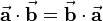
On the basis of the described relations it appears, that the commutative law holds:
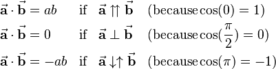
Furthermore the following special cases can be considered, that often lead to simplifications in technical context:
Multimedial educational material
|
|
http://demonstrations.wolfram.com/DotProduct/ Applet: Dot product of two vectors (free CDF-Player required) |

Literature
- Kurt Meyberg und Peter Vachenauer, Höhere Mathematik 1: Differential- und Integralrechnung. Vektor- und Matrizenrechnung, 6. Edition (Springer Berlin Heidelberg, 2001)
- Manfred Albach, Grundlagen der Elektrotechnik 1: Erfahrungssätze, Bauelemente, Gleichstromschaltungen, 3. Edition (Pearson Studium, 2011)