Rotations using quaternions
| ← Back: Multiplication of quaternions | Overview: Quaternions | Next: Composition of rotations → |

Usually rotations are defined by 3 angles, either Euler or Roll-Pitch-Yaw angles. So three successive rotations around three different axes lead to a combined rotation, that can be described by a single rotation matrix. Such a combined rotation is equal to a rotation around a certain axis in three-dimensional space about a certain angle. This is shown in the figure on the right. The vector  is rotated such that it results in
  . This could be done by rotating the vector around the z-, the y- and the x-axis successively or by just rotating it around the rotation axis
  by
by  .
.
Mathematical description
First the rotation axis has to be defined by a unit vector. So it holds:

Then a rotation about by the angle can be represented by a quaternion  like follows:
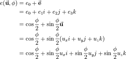
So the scalar part  is defined as the cosine of
  and the vector part consisting of
  ,
,  and
and  equals multiplied by the sine of .
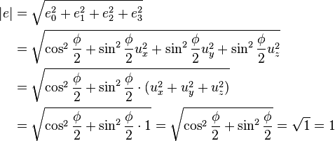
That the resulting quaternion is a unit quaternion can be proven as follows:
So if a quaternion  is given, the angle and the rotation axis can be computed as follows:
![\begin{align}
\phi &= 2\cdot \arccos e_0 \\
\vec{\mathbf{u}} &= \frac{1}{\sin{\frac{\phi}{2}}}\left[\begin{array}{c}e_1\\e_2\\e_3\end{array}\right]
\end{align}](/wiki/robotics/images/math/1/e/7/1e72499fe5dbe6181daca882d56bad8b.png)
Mathematical solving of a quaternion rotation
Assume a quaternion  describing a rotation and a vector that should be rotated. To be able to apply the rotation, has to be presented as a quaternion. So the pure quaternion
  is defined with scalar part equal to 0 and as vector part:

The same is done for the resulting vector  of the rotation:

The rotation is then applied by the following quaternion multiplication:
Following the rules for quaternion multiplication, this equation leads to
![r' = e \ r \ e^* = 0 \ \oplus \
\left[\begin{array}{ccc}
e_0^2+e_1^2-e_2^2-e_3^2 & 2(e_1e_2-e_0e_3) & 2(e_0e_2+e_1e_3) \\
2(e_0e_3+e_1e_2) & e_0^2-e_1^2+e_2^2-e_3^2 & 2(e_2e_3-e_0e_1) \\
2(e_1e_3-e_0e_2) & 2(e_0e_1+e_2e_3) & e_0^2-e_1^2-e_2^2+e_3^2
\end{array}\right]
\left[\begin{array}{ccc}
r_1 \\
r_2 \\
r_3
\end{array}\right]
= 0 \ \oplus \ \mathbf{R_e}\vec{\mathbf{r}}](/wiki/robotics/images/math/d/4/5/d45fee89f4f65b4d9781f404729ebb99.png)
This shows, that the result of the multiplication is again a pure quaternion describing the rotated vector . The corresponding rotation matrix describing the rotation obtained by the quaternion can easily be computed using the equation for  .
.
How several rotations can be composed in one quaternion is explained in the next article Composition of rotations.
 An object is shifted 1 unit on the x-axis. So its position vector and the corresponding quaternion are defined as follows: Assume the object or the vector, respectively, is rotated corresponding to the Roll-Pitch-Yaw notation like shown in the figure on the right. So the first rotation is applied around the z-axis by a yaw angle of The resulting vector Regarding the figure it can easily be seen, that a rotation around the diagonal Using the quaternion rotation equation So the rotation matrices for the rotation done following the Roll-Pitch-Yaw rule and the corresponding rotation using a quaternion lead to the same rotation matrices The applet at the bottom of this page can be used to reconstruct the example situation and to test other combinations of roll, pitch and yaw angle and the corresponding quaternions. |
![\vec{\mathbf{p}} = \left[\begin{array}{c}1\\0\\0\end{array}\right], \qquad
p = 0 \ \oplus \ \vec{\mathbf{p}} = (0,1,0,0)](/wiki/robotics/images/math/4/6/2/462081f9a2124f4f740bbe142878f0ed.png)
 (shown in blue). Then it is rotated around the y-axis by a pitch angle of
  (shown in green). The roll angle is defined as
  around the x-axis (shown in red). Multiplying the three rotation matrices leads to the following combined rotation matrix:
![\begin{align}
\mathbf{R}_{rpy} &=
\left[\begin{array}{ccc}
1 & 0 & 0 \\
0 & \cos{45^\circ} & -\sin{45^\circ} \\
0 & \sin{45^\circ} & \cos{45^\circ}
\end{array}\right]
\left[\begin{array}{ccc}
\cos{90^\circ} & 0 & \sin{90^\circ} \\
0 & 1 & 0 \\
-\sin{90^\circ} & 0 & \cos{90^\circ}
\end{array}\right]
\left[\begin{array}{ccc}
\cos{135^\circ} & -\sin{135^\circ} & 0 \\
\sin{135^\circ} & \cos{135^\circ} & 0 \\
0 & 0 & 1
\end{array}\right]
\\ &=
\left[\begin{array}{ccc}
1 & 0 & 0 \\
0 & \frac{1}{\sqrt{2}} & -\frac{1}{\sqrt{2}} \\
0 & \frac{1}{\sqrt{2}} & \frac{1}{\sqrt{2}}
\end{array}\right]
\left[\begin{array}{ccc}
0 & 0 & 1 \\
0 & 1 & 0 \\
-1 & 0 & 0
\end{array}\right]
\left[\begin{array}{ccc}
-\frac{1}{\sqrt{2}} & -\frac{1}{\sqrt{2}} & 0 \\
\frac{1}{\sqrt{2}} & -\frac{1}{\sqrt{2}} & 0 \\
0 & 0 & 1
\end{array}\right]
\\ &=
\left[\begin{array}{ccc}
0 & 0 & 1 \\
0 & -1 & 0 \\
1 & 0 & 0
\end{array}\right]
\end{align}](/wiki/robotics/images/math/a/9/0/a90ef71964c007db247e2d570170884c.png)
 of the rotation, that is also shown in the figure on the right, then is:
![\begin{align}
\vec{\mathbf{p'}} = \mathbf{R}_{rpy}\vec{\mathbf{p}} = \left[\begin{array}{ccc}
0 & 0 & 1 \\
0 & -1 & 0 \\
1 & 0 & 0
\end{array}\right]
\left[\begin{array}{c}1\\0\\0\end{array}\right] = \left[\begin{array}{c}0\\0\\1\end{array}\right]
\end{align}](/wiki/robotics/images/math/d/7/7/d77e4be771da0b3d17d84bf023cabee5.png)
 results in the same vector
  is
is  . So this rotation can be described by a quaternion
 ![\begin{align}
e(\vec{\mathbf{u}},180^\circ) &= \cos{\frac{180^\circ}{2}}+\sin{\frac{180^\circ}{2}}\vec{\mathbf{u}} =
\cos{\frac{180^\circ}{2}}+\sin{\frac{180^\circ}{2}}\left[\begin{array}{c}\frac{1}{\sqrt{2}}\\ 0\\\frac{1}{\sqrt{2}}\end{array}\right]=
0 + \frac{1}{\sqrt{2}}i + 0\ j + \frac{1}{\sqrt{2}}k \\
&= (0,\frac{1}{\sqrt{2}},0,\frac{1}{\sqrt{2}})
\end{align}](/wiki/robotics/images/math/6/6/8/668def1d9cafbea7adafce1b0e48006e.png)
 and solving it then leads to:
![\begin{align}
p' = e \ p \ e^* &= 0 \ \oplus \ \mathbf{R_e}\vec{\mathbf{p}}
\\ &= 0 \ \oplus \
\left[\begin{array}{ccc}
e_0^2+e_1^2-e_2^2-e_3^2 & 2(e_1e_2-e_0e_3) & 2(e_0e_2+e_1e_3) \\
2(e_0e_3+e_1e_2) & e_0^2-e_1^2+e_2^2-e_3^2 & 2(e_2e_3-e_0e_1) \\
2(e_1e_3-e_0e_2) & 2(e_0e_1+e_2e_3) & e_0^2-e_1^2-e_2^2+e_3^2
\end{array}\right]
\left[\begin{array}{c}
p_1 \\
p_2 \\
p_3
\end{array}\right]
\\ &= 0 \ \oplus \
\left[\begin{array}{ccc}
0^2+\frac{1}{\sqrt{2}}^2-0^2-\frac{1}{\sqrt{2}}^2 & 2(\frac{1}{\sqrt{2}}\cdot 0-0\cdot \frac{1}{\sqrt{2}}) & 2(0 \cdot 0+\frac{1}{\sqrt{2}} \cdot \frac{1}{\sqrt{2}}) \\
2(0\cdot \frac{1}{\sqrt{2}}+\frac{1}{\sqrt{2}} \cdot 0) & 0^2-\frac{1}{\sqrt{2}}^2+0^2-\frac{1}{\sqrt{2}}^2 & 2(0 \cdot \frac{1}{\sqrt{2}}-0 \cdot \frac{1}{\sqrt{2}}) \\
2(\frac{1}{\sqrt{2}} \cdot \frac{1}{\sqrt{2}}-0 \cdot 0) & 2(0 \cdot \frac{1}{\sqrt{2}}+0 \cdot \frac{1}{\sqrt{2}}) & 0^2-\frac{1}{\sqrt{2}}^2-0^2+\frac{1}{\sqrt{2}}^2
\end{array}\right]
\left[\begin{array}{c}
p_1 \\
p_2 \\
p_3
\end{array}\right]
\\ &= 0 \ \oplus \
\left[\begin{array}{ccc}
0+\frac{1}{2}-0-\frac{1}{2} & 2\cdot 0 & 2(0 +\frac{1}{2}) \\
2\cdot 0 & 0-\frac{1}{2}+0-\frac{1}{2} & 2 \cdot 0 \\
2(\frac{1}{2}-0) & 2 \cdot 0 & 0-\frac{1}{2}-0+\frac{1}{2}
\end{array}\right]
\left[\begin{array}{c}
p_1 \\
p_2 \\
p_3
\end{array}\right]
\\ &= 0 \ \oplus \
\left[\begin{array}{ccc}
0 & 0 & 1 \\
0 & -1 & 0 \\
1 & 0 & 0
\end{array}\right]
\left[\begin{array}{c}
p_1 \\
p_2 \\
p_3
\end{array}\right]
\end{align}](/wiki/robotics/images/math/0/f/6/0f655dff38951e3377814529bc190be6.png)
 and
and  and so to the same vector
 Applet
The following three-dimensional applet helps you to understand the relation between Roll-Pitch-Yaw angles and a quaternion. The initial position of the object can be set using the sliders for x, y and z. Then the object can be rotated by defining the roll, pitch and yaw angles. The most intuitive way is to start with the yaw angle, because this one is applied first. Then the object is rotated aroud the y-axis by the pitch angle followed by a rotation around the x-axis by the roll angle. The quaternion describing the same rotation is shown dynamically and the corresponding angle  and the rotation axis are presented. The rotation axis and the rotational path are visualized on the left side. After pressing the Show Quaternion Rotation button, the rotation of the object around gets animated.