Simple arithmetic operations

← Back: Unit vectors

Overview: Vector algebra

Next: Dot product →

Addition and subtraction of vectors

Vectors can be added graphically as well as computationally. Using the graphical method, one of the vectors is shifted such that its startpoint is positioned at the endpoint of the other vector. The resulting vector is called sum vector. It starts at the startpoint the one vector and ends at the endpoint of the shifted vector (see figure on the right). For the computational addition the single components are added

$\vec{\mathbf{a}} + \vec{\mathbf{b}} = \begin{bmatrix} a_x\\a_y\\a_z \end{bmatrix} + \begin{bmatrix} b_x\\b_y\\b_z \end{bmatrix} = \begin{bmatrix} a_x+b_x\\a_y+b_y\\a_z+b_z \end{bmatrix}$

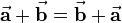
Both the graphical and the computational addition show, that the commutative law holds:

$\vec{\mathbf{a}}+\vec{\mathbf{b}} = \vec{\mathbf{b}}+\vec{\mathbf{a}}$

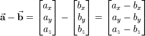
The resulting vector of the substraction of vectors is called difference vector. Because 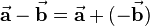$\vec{\mathbf{a}}-\vec{\mathbf{b}} = \vec{\mathbf{a}}+(-\vec{\mathbf{b}})$ the two vectors can just be added after inverting the direction of the second vector (see figure on the right). For the computational method the components are substracted:

$\vec{\mathbf{a}} - \vec{\mathbf{b}} = \begin{bmatrix} a_x\\a_y\\a_z \end{bmatrix} - \begin{bmatrix} b_x\\b_y\\b_z \end{bmatrix} = \begin{bmatrix} a_x-b_x\\a_y-b_y\\a_z-b_z \end{bmatrix}$

If more than two vectors are added or substracted the same relations hold. Using the graphical method for example, all the vectors are stringed together.

Multiplication of vectors with scalars

Bei der Multiplikation eines Vektors $\vec{\textbf{a}}$ mit einem positiven reellen Skalar $\lambda$ erhält man einen neuen Vektor, dessen Richtung mit derjenigen des ursprünglichen Vektors übereinstimmt. Bei der Multiplikation eines Vektors $\vec{\textbf{a}}$ mit einem negativen reellen Skalar $\lambda$ erhält man einen Vektor mit entgegengesetzter Richtung. Die Länge des neuen Vektors ändert sich in beiden Fällen um den Faktor $|\lambda|$. 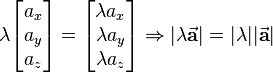Dies wird sofort anhand der mathematischen Bestimmung des neuen Vektors ersichtlich, bei der jede Komponente des Vektors mit dem Skalar multipliziert wird:

$\lambda \begin{bmatrix} a_x\\a_y\\a_z \end{bmatrix} = \begin{bmatrix} \lambda a_x\\ \lambda a_y\\ \lambda a_z \end{bmatrix} \Rightarrow |\lambda \vec{\textbf{a}}| = |\lambda| |\vec{\textbf{a}}|$

Bei der Multiplikation mit einem Skalar $\lambda = 0$ erhält man als Sonderfall den Nullvektor $\vec{\textbf{0}}$ mit dem Betrag $0$ und unbestimmter Richtung. Ein praktisches Beispiel für die Multiplikation eines Vektors mit einem Skalar findet sich in der Einführung in die Vektorrechnung.

Multimedial educational material

http://mathcasts.org/gg/student/matrices/vectors_adding/index_s.html Applet: Vector addition in cartesian coordinates http://demonstrations.wolfram.com/VectorsIn3D/ Applet: Vector addition in three-dimensional space (free CDF-Player of Wolfram required) http://demonstrations.wolfram.com/3DVectorDecomposition/ Applet: Vector addition in in three-dimensional space with three vectors (free CDF-Player required) http://www.math.ethz.ch/~lemuren/public/visualization/analysis/RealComputation.html Applet: Vector addition in two-dimensional space http://demonstrations.wolfram.com/SumOfTwoVectors/ Applet: Vector addition in cartesian coordinates (free CDF-Player of Wolfram required)

Helpful links

http://hyperphysics.phy-astr.gsu.edu/hbase/vect.html General introduction to vector operations