Difference between revisions of "Dot product"
| Line 10: | Line 10: | ||
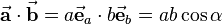
Regarding the right side of the above equation, the following correlation can be noted: If you project the vector <math>\vec{\mathbf{b}}</math> on the vector <math>\vec{\mathbf{a}}</math>, you get the distance <math>b\cos\alpha</math>. As a consequence the result of the dot product can be seen as the acreage of a rectangle with the side legths <math>a</math> and <math>b\cos\alpha</math>. The projection can also be done contrariwise (projection of vector <math>\vec{\mathbf{a}}</math> on the direction of vector <math>\vec{\mathbf{b}}</math>). So that you get the distance <math>a\cos\alpha</math>. The multiplication of this term with <math>b</math> leads to a rectangle with equivalent acreage but different aspect ratio (see figure). | Regarding the right side of the above equation, the following correlation can be noted: If you project the vector <math>\vec{\mathbf{b}}</math> on the vector <math>\vec{\mathbf{a}}</math>, you get the distance <math>b\cos\alpha</math>. As a consequence the result of the dot product can be seen as the acreage of a rectangle with the side legths <math>a</math> and <math>b\cos\alpha</math>. The projection can also be done contrariwise (projection of vector <math>\vec{\mathbf{a}}</math> on the direction of vector <math>\vec{\mathbf{b}}</math>). So that you get the distance <math>a\cos\alpha</math>. The multiplication of this term with <math>b</math> leads to a rectangle with equivalent acreage but different aspect ratio (see figure). | ||
| − | + | Another possibility to compute the dot product is to multiply the corresponding components and sum them up: | |
:<math> | :<math> | ||
| − | \vec{\ | + | \vec{\mathbf{a}} \cdot \vec{\mathbf{b}} = a b\cos\alpha = a_x b_x + a_y b_y + a_z b_z |
</math> | </math> | ||
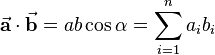
Ganz allgemein - zum Beispiel wenn man es nicht mit Vektoren aus dem kartesischen Koordinatensystem zu tun hat - lässt sich das Skalarprodukt wie folgt bestimmen: | Ganz allgemein - zum Beispiel wenn man es nicht mit Vektoren aus dem kartesischen Koordinatensystem zu tun hat - lässt sich das Skalarprodukt wie folgt bestimmen: | ||
:<math> | :<math> | ||
| − | \vec{\ | + | \vec{\mathbf{a}} \cdot \vec{\mathbf{b}} = a b \cos\alpha = \sum_{i=1}^{n} a_i b_i |
</math> | </math> | ||
Anhand der beschriebenen Zusammenhänge zeigt sich, dass das Skalarprodukt dem Kommutativgesetz genügt. Somit gilt: | Anhand der beschriebenen Zusammenhänge zeigt sich, dass das Skalarprodukt dem Kommutativgesetz genügt. Somit gilt: | ||
:<math> | :<math> | ||
| − | \vec{\ | + | \vec{\mathbf{a}} \cdot \vec{\mathbf{b}} = \vec{\mathbf{b}} \cdot \vec{\mathbf{a}} |
</math> | </math> | ||
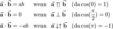
Weiterhin ergeben sich einige Sonderfälle, die im technischen Kontext häufig zu Vereinfachungen führen: | Weiterhin ergeben sich einige Sonderfälle, die im technischen Kontext häufig zu Vereinfachungen führen: | ||
:<math> | :<math> | ||
\begin{align} | \begin{align} | ||
| − | \vec{\ | + | \vec{\mathbf{a}} \cdot \vec{\mathbf{b}} &= ab& |
&\text{wenn}& | &\text{wenn}& | ||
| − | \vec{\ | + | \vec{\mathbf{a}} & \upuparrows \vec{\mathbf{b}}& &(\text{da} \cos(0) = 1)\\ |
| − | \vec{\ | + | \vec{\mathbf{a}} \cdot \vec{\mathbf{b}} &= 0& |
&\text{wenn}& | &\text{wenn}& | ||
| − | \vec{\ | + | \vec{\mathbf{a}} &\perp \vec{\mathbf{b}}& &(\text{da} \cos(\frac{\pi}{2}) = 0)\\ |
| − | \vec{\ | + | \vec{\mathbf{a}} \cdot \vec{\mathbf{b}} &= -ab& |
&\text{wenn}& | &\text{wenn}& | ||
| − | \vec{\ | + | \vec{\mathbf{a}} &\downarrow\uparrow \vec{\mathbf{b}}& &(\text{da} \cos(\pi) = -1) |
\end{align} | \end{align} | ||
</math> | </math> | ||
| Line 40: | Line 40: | ||
|Title=Arbeit im elektrischen Feld | |Title=Arbeit im elektrischen Feld | ||
|Contents= | |Contents= | ||
| − | Ein häufiger Anwendungsfall des Skalarprodukts ergibt sich bei dem Begriff der Arbeit. Bewegt man beispielsweise eine Punktladung <math>Q</math> in einem homogenen elektrischen Feld <math>\vec{\ | + | Ein häufiger Anwendungsfall des Skalarprodukts ergibt sich bei dem Begriff der Arbeit. Bewegt man beispielsweise eine Punktladung <math>Q</math> in einem homogenen elektrischen Feld <math>\vec{\mathbf{E}}</math> entlang einer geraden Strecke <math>\vec{\mathbf{s}}</math> von einem Punkt <math>A</math> zu einem Punkt <math>B</math>, so lässt sich die dabei aufgewendete Arbeit mit Hilfe des Skalarprodukts wie folgt bestimmen: |
:<math> | :<math> | ||
| − | W_{AB} = \vec{\ | + | W_{AB} = \vec{\mathbf{F}} \cdot \vec{\mathbf{s}} |
</math> | </math> | ||
| − | Bei der Verschiebung der Ladung muss die Coulomb-Kraft <math>\vec{\ | + | Bei der Verschiebung der Ladung muss die Coulomb-Kraft <math>\vec{\mathbf{F}} = Q\vec{\mathbf{E}}</math> aufgebracht werden, das heißt in diesem Fall ergibt sich der folgende Zusammenhang: |
:<math> | :<math> | ||
| − | W_{AB} = Q\vec{\ | + | W_{AB} = Q\vec{\mathbf{E}} \cdot \vec{\mathbf{s}} = Q E \cos{\alpha} |
</math> | </math> | ||
Allgemein, also wenn die elektrische Feldstärke nicht homogen und der Weg der Verschiebung von <math>A</math> nach <math>B</math> keine gerade Strecke ist, gilt: | Allgemein, also wenn die elektrische Feldstärke nicht homogen und der Weg der Verschiebung von <math>A</math> nach <math>B</math> keine gerade Strecke ist, gilt: | ||
:<math> | :<math> | ||
| − | W_{AB} = \int_{A}^{B} \vec{\ | + | W_{AB} = \int_{A}^{B} \vec{\mathbf{F}} \cdot \mathrm{d}\vec{\mathbf{s}} = Q \int_{A}^{B} \vec{\mathbf{E}} \cdot \mathrm{d}\vec{\mathbf{s}} |
</math> | </math> | ||
}} | }} | ||
Revision as of 13:27, 15 May 2014
| ← Back: Simple arithmetic operations | Overview: Vector algebra | Next: Cross product → |

The dot product of two vectors results in a scalar value and is defined as
where  describes the angle between the two vectors which ranges from
  to
to  (see figure). The dot product is denoted with a simple point between the vectors or without any sign.
Regarding the right side of the above equation, the following correlation can be noted: If you project the vector  on the vector
  , you get the distance
  . As a consequence the result of the dot product can be seen as the acreage of a rectangle with the side legths
  and . The projection can also be done contrariwise (projection of vector on the direction of vector ). So that you get the distance
  . The multiplication of this term with
  leads to a rectangle with equivalent acreage but different aspect ratio (see figure).
Another possibility to compute the dot product is to multiply the corresponding components and sum them up:

Ganz allgemein - zum Beispiel wenn man es nicht mit Vektoren aus dem kartesischen Koordinatensystem zu tun hat - lässt sich das Skalarprodukt wie folgt bestimmen:
Anhand der beschriebenen Zusammenhänge zeigt sich, dass das Skalarprodukt dem Kommutativgesetz genügt. Somit gilt:
Weiterhin ergeben sich einige Sonderfälle, die im technischen Kontext häufig zu Vereinfachungen führen:
Ein häufiger Anwendungsfall des Skalarprodukts ergibt sich bei dem Begriff der Arbeit. Bewegt man beispielsweise eine Punktladung Bei der Verschiebung der Ladung muss die Coulomb-Kraft Allgemein, also wenn die elektrische Feldstärke nicht homogen und der Weg der Verschiebung von |
 in einem homogenen elektrischen Feld
  entlang einer geraden Strecke
  von einem Punkt
  zu einem Punkt
  , so lässt sich die dabei aufgewendete Arbeit mit Hilfe des Skalarprodukts wie folgt bestimmen:
 aufgebracht werden, das heißt in diesem Fall ergibt sich der folgende Zusammenhang:
Multimedial educational material
|
|
http://www.mathresource.iitb.ac.in/linear%20algebra/example7.1/index.html Applet: Skalarprodukt zweier Vektoren (engl.) http://www.cs.brown.edu/exploratories/freeSoftware/repository/edu/brown/cs/exploratories/applets/dotProduct/dot_product_java_browser.html Applet: Skalarprodukt zweier Vektoren http://www.mathresource.iitb.ac.in/linear%20algebra/example7.2/index.html Applet: Skalarprodukt zweier Vektoren mit der eingeschlossenen Fläche http://demonstrations.wolfram.com/DotProduct/ Applet: Skalarprodukt zweier Vektoren (engl./ free CDF-Player erforderlich) http://www.math.ethz.ch/~lemuren/public/exercise/linalg/LinearCombinationInR2ETHZ.html Applet: Linearkombination im zweidimensionalem Raum |

Literature
- Kurt Meyberg und Peter Vachenauer, Höhere Mathematik 1: Differential- und Integralrechnung. Vektor- und Matrizenrechnung, 6. Edition (Springer Berlin Heidelberg, 2001)
- Manfred Albach, Grundlagen der Elektrotechnik 1: Erfahrungssätze, Bauelemente, Gleichstromschaltungen, 3. Edition (Pearson Studium, 2011)