Matrix inversion

Matrix inversion

The inverse of an n-by-n square matrix $\mathbf{A}$ is denoted as $\mathbf{A}^{-1}$ and defined such that

$\mathbf{A}\mathbf{A}^{-1}=\mathbf{A}^{-1}\mathbf{A}=\mathbf{I}_n$

where $\mathbf{I}_n$ is the n-by-n identity matrix.
Prerequesite for the inversion is, that $\mathbf{A}$ is an n-by-n square matrix and that $\mathbf{A}$ is regular. Regular means that the row and column vectors are linearly independent and so the determinant is nonzero:

$det(\mathbf{A})\ne0$

Otherwise the matrix is called singular.

 Example: 

 $\mathbf{A}_e  = 
\left[\begin{array}{cccc}
1 & 2 & 0 & 0\\
3 & 0 & 1 & 1\\
0 & 1 & 0 & 0\\
0 & 0 & 2 & 1
\end{array}\right]
,\quad
\mathbf{A}_e^{-1}  = 
\left[\begin{array}{cccc}
1 & 0 & -2 & 0\\
0 & 0 & 1 & 0\\
3 & -1 & -6 & 1\\
-6 & 2 & 12 & -1
\end{array}\right]$


 $\begin{align}
\mathbf{A}_e\mathbf{A}_e^{-1}  &= 
\left[\begin{array}{cccc}
1 & 2 & 0 & 0\\
3 & 0 & 1 & 1\\
0 & 1 & 0 & 0\\
0 & 0 & 2 & 1
\end{array}\right]\cdot
\left[\begin{array}{cccc}
1 & 0 & -2 & 0\\
0 & 0 & 1 & 0\\
3 & -1 & -6 & 1\\
-6 & 2 & 12 & -1
\end{array}\right]\\&=
\left[\begin{array}{cccc}
1+0+0+0 & 0+0+0+0 & -2+2+0+0 & 0+0+0+0\\
3+0+3-6 & 0+0-1+2 & -6+0-6+12 & 0+0+1-1\\
0+0+0+0 & 0+0+0+0 & 0+1+0+0 & 0+0+0+0\\
0+0+6-6 & 0+0-2+2 & 0+0-12+12 & 0+0+2-1
\end{array}\right]\\&=
\left[\begin{array}{cccc}
1 & 0 & 0 & 0\\
0 & 1 & 0 & 0\\
0 & 0 & 1 & 0\\
0 & 0 & 0 & 1
\end{array}\right]=
\mathbf{I}_n
\end{align}$

Before determining the inverse of a matrix it is always useful to compute the determinant and check whether the matrix is regular or singular. If it is singular it is not possible to determine the inverse because there is no inverse. For 3-by-3 and smaller matrices there are simple formulas to compute the determinant. To compute the determinant of larger matrices the following paragraph describes an example formula for a 4-by-4 matrix.

To determine the inverse of a matrix there are several alternatives. Two of the common procedures are the Gauß-Jordan-Algorithm and the Adjugate Formula that are explained afterwards.

Determinant of a 4-by-4 matrix

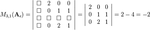
This paragraph describes a formula to compute the determinant of a 4-by-4 matrix using minors and cofactors of a matrix.

The minor $M_{i,j}(\mathbf{A})$ of an n-by-n square matrix $\mathbf{A}$ is the determinant of a smaller square matrix obtained by removing the row $i$ and the column $j$ from $\mathbf{A}$.

 The minors $M_{1,4}(\mathbf{A}_e)$ and $M_{3,1}(\mathbf{A}_e)$ for example are defined as


 $M_{1,4}(\mathbf{A}_e)=
\left|\begin{array}{cccc}
\Box & \Box & \Box & \Box\\
3 & 0 & 1 & \Box\\
0 & 1 & 0 & \Box\\
0 & 0 & 2 & \Box
\end{array}\right|=
\left|\begin{array}{ccc}
3 & 0 & 1\\
0 & 1 & 0\\
0 & 0 & 2
\end{array}\right|=6-0=6$

 $M_{3,1}(\mathbf{A}_e)=
\left|\begin{array}{cccc}
\Box & 2 & 0 & 0\\
\Box & 0 & 1 & 1\\
\Box & \Box & \Box & \Box\\
\Box & 0 & 2 & 1
\end{array}\right|=
\left|\begin{array}{ccc}
2 & 0 & 0\\
0 & 1 & 1\\
0 & 2 & 1
\end{array}\right|=2-4=-2$

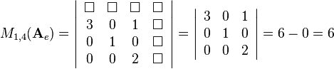
Multiplying the minor with $(-1)^{i+j}$ results in the cofactor $C_{i,j}(\mathbf{A})$:

$C_{i,j}(\mathbf{A})=(-1)^{i+j}M_{i,j}(\mathbf{A})$

 $C_{1,4}(\mathbf{A}_e)=(-1)^{1+4}M_{1,4}(\mathbf{A}_e)=(-1)^5\cdot6=-6$

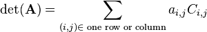
To compute the determinant of matrix $\mathbf{A}$ first one row or column is choosen. The sum of the four corresponding values of the row or column multiplied by the related cofactors results in the determinant:

$\det(\mathbf{A})=\sum_{(i,j) \isin \text{ one row or column}}{a_{i,j}C_{i,j}}$

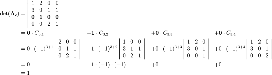
 For the example matrix it is useful to choose the row 3 because it contains three zero values as factors:

 $\begin{align}
\det(\mathbf{A}_e)&=
\left|\begin{array}{cccc}
1 & 2 & 0 & 0\\
3 & 0 & 1 & 1\\
\mathbf{0} & \mathbf{1} & \mathbf{0} & \mathbf{0}\\
0 & 0 & 2 & 1
\end{array}\right| & \quad & \quad & \quad\\
&=
\mathbf{0}\cdot C_{3,1}&+&\mathbf{1}\cdot C_{3,2}&+&\mathbf{0}\cdot C_{3,3}&+&\mathbf{0}\cdot C_{3,4}\\
&=
0\cdot(-1)^{3+1}
\left|\begin{array}{ccc}
2 & 0 & 0\\
0 & 1 & 1\\
0 & 2 & 1
\end{array}\right|
&+&1\cdot(-1)^{3+2}
\left|\begin{array}{ccc}
1 & 0 & 0\\
3 & 1 & 1\\
0 & 2 & 1
\end{array}\right|
&+&0\cdot(-1)^{3+3}
\left|\begin{array}{ccc}
1 & 2 & 0\\
3 & 0 & 1\\
0 & 0 & 1
\end{array}\right|
&+&0\cdot(-1)^{3+4}
\left|\begin{array}{ccc}
1 & 2 & 0\\
3 & 0 & 1\\
0 & 0 & 2
\end{array}\right|\\
&= 0&+&1\cdot(-1)\cdot(-1)&+&0&+&0\\
&= 1&\quad&\quad&\quad
\end{align}$

Gauß-Jordan-Algorithm

The Gauß-Jordan-Algorithm was developed to solve systems of linear equations. But it can also be used to determine the inverse of an n-by-n square matrix.

The algorithm is based on the formula $\mathbf{A}\mathbf{A}^{-1}=\mathbf{I}_n$. First the block matrix $(\mathbf{A}|\mathbf{I}_n)$ is build. On this matrix the Gauß-Jordan-Algorithm is applied. By using various conversion steps like interchanging of rows and addtition of factorized rows to other rows the block matrix is converted so that the left block equals the identity matrix $\mathbf{I}_n$. The right block then corresponds to the inverse of $\mathbf{A}$.

Gauß-Jordan-Algorithm

 $\begin{align}
(\mathbf{A}_e|\mathbf{I}_n) = 
&\left[\begin{array}{cccc|cccc}
1 & 2 & 0 & 0 & 1 & 0 & 0 & 0\\
3 & 0 & 1 & 1 & 0 & 1 & 0 & 0\\
0 & 1 & 0 & 0 & 0 & 0 & 1 & 0\\
0 & 0 & 2 & 1 & 0 & 0 & 0 & 1
\end{array}\right]\\ \\
&\text{--------------------------------------------------------------------------------------}\\ \\
&\left[\begin{array}{cccc|cccc}
1 & 2 & 0 & 0 & 1 & 0 & 0 & 0\\
3 & 0 & 1 & 1 & 0 & 1 & 0 & 0\\
0 & 1 & 0 & 0 & 0 & 0 & 1 & 0\\
0 & 0 & 2 & 1 & 0 & 0 & 0 & 1
\end{array}\right]
\begin{array}{c}
\\
\updownarrow\text{interchange row II and row III}\\
\\
\end{array}\\
&\qquad\qquad\quad\quad\Downarrow\\
&\left[\begin{array}{cccc|cccc}
1 & 2 & 0 & 0 & 1 & 0 & 0 & 0\\
0 & 1 & 0 & 0 & 0 & 0 & 1 & 0\\
3 & 0 & 1 & 1 & 0 & 1 & 0 & 0\\
0 & 0 & 2 & 1 & 0 & 0 & 0 & 1
\end{array}\right]
\begin{array}{c}
\text{substract 2 times row II}\\
\\
\\
\\
\end{array}\\
&\qquad\qquad\quad\quad\Downarrow\\
&\left[\begin{array}{cccc|cccc}
1 & 0 & 0 & 0 & 1 & 0 & -2 & 0\\
0 & 1 & 0 & 0 & 0 & 0 & 1 & 0\\
3 & 0 & 1 & 1 & 0 & 1 & 0 & 0\\
0 & 0 & 2 & 1 & 0 & 0 & 0 & 1
\end{array}\right]
\begin{array}{c}
\\
\\
\text{substract 3 times row I}\\
\\
\end{array}\\
&\qquad\qquad\quad\quad\Downarrow\\
&\left[\begin{array}{cccc|cccc}
1 & 0 & 0 & 0 & 1 & 0 & -2 & 0\\
0 & 1 & 0 & 0 & 0 & 0 & 1 & 0\\
0 & 0 & 1 & 1 & -3 & 1 & 6 & 0\\
0 & 0 & 2 & 1 & 0 & 0 & 0 & 1
\end{array}\right]
\begin{array}{c}
\\
\\
\updownarrow\text{interchange row III and row IV}\\
\end{array}\\
&\qquad\qquad\quad\quad\Downarrow\\
&\left[\begin{array}{cccc|cccc}
1 & 0 & 0 & 0 & 1 & 0 & -2 & 0\\
0 & 1 & 0 & 0 & 0 & 0 & 1 & 0\\
0 & 0 & 2 & 1 & 0 & 0 & 0 & 1\\
0 & 0 & 1 & 1 & -3 & 1 & 6 & 0
\end{array}\right]
\begin{array}{c}
\\
\\
\text{substract row IV}\\
\\
\end{array}\\
&\qquad\qquad\quad\quad\Downarrow\\
&\left[\begin{array}{cccc|cccc}
1 & 0 & 0 & 0 & 1 & 0 & -2 & 0\\
0 & 1 & 0 & 0 & 0 & 0 & 1 & 0\\
0 & 0 & 1 & 0 & 3 & -1 & -6 & 1\\
0 & 0 & 1 & 1 & -3 & 1 & 6 & 0
\end{array}\right]
\begin{array}{c}
\\
\\
\\
\text{substract row III}\\
\end{array}\\
&\qquad\qquad\quad\quad\Downarrow\\
&\left[\begin{array}{cccc|cccc}
{\color{Green}\mathbf{1}} & 0 & 0 & 0 & 1 & 0 & -2 & 0\\
0 & {\color{Green}\mathbf{1}} & 0 & 0 & 0 & 0 & 1 & 0\\
0 & 0 & {\color{Green}\mathbf{1}} & 0 & 3 & -1 & -6 & 1\\
0 & 0 & 0 & {\color{Green}\mathbf{1}} & -6 & 2 & 12 & -1
\end{array}\right]\\ 
&\qquad\quad\mathbf{I}_n\qquad\qquad\qquad\mathbf{A}_e^{-1}\\ \\
&\text{--------------------------------------------------------------------------------------}\\ \\
\mathbf{A}_e^{-1}  = 
&\left[\begin{array}{cccc}
1 & 0 & -2 & 0\\
0 & 0 & 1 & 0\\
3 & -1 & -6 & 1\\
-6 & 2 & 12 & -1
\end{array}\right]
\end{align}$

Adjugate Formula

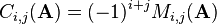
The adjugate formula defines the inverse of an n-by-n square matrix $\mathbf{A}$ as

$\mathbf{A}^{-1}=\frac{1}{\det(\mathbf{A})}\text{adj}(\mathbf{A})$

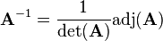
where $\text{adj}(\mathbf{A})$ is the so called adjugate matrix of $\mathbf{A}$. The adjugate matrix is the transposed of the cofactor matrix:

$\text{adj}(\mathbf{A})=\mathbf{C}(\mathbf{A})^T$

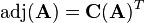
And the cofactor matrix $\mathbf{C}(\mathbf{A})$ is just a matrix where each cell corresponds to the related cofactor:

$\mathbf{C}(\mathbf{A})=\left[\begin{array}{cccc} C_{1,1}(\mathbf{A}) & C_{1,2}(\mathbf{A}) & \cdots & C_{1,n}(\mathbf{A})\\ C_{2,1}(\mathbf{A}) & C_{2,2}(\mathbf{A}) & & C_{2,n}(\mathbf{A})\\ \vdots & & \ddots & \vdots\\ C_{n,1}(\mathbf{A}) & C_{n,2}(\mathbf{A}) & \cdots & C_{n,n}(\mathbf{A}) \end{array}\right]$

So to determine the inverse of an n-by-n square matrix you have to compute the n square cofactors, then transpose the resulting cofactor matrix and divide all the values by the determinant.

 $\begin{align}
\mathbf{C}(\mathbf{A}_e)&=
\left[\begin{array}{cccc}
1 & 0 & 3 & -6\\
0 & 0 & -1 & 2\\
-2 & 1 & -6 & 12\\
0 & 0 & 1 & -1
\end{array}\right]\\ \\
\mathbf{C}(\mathbf{A}_e)^T&=
\left[\begin{array}{cccc}
1 & 0 & -2 & 0\\
0 & 0 & 1 & 0\\
3 & -1 & -6 & 1\\
-6 & 2 & 12 & -1
\end{array}\right]=\text{adj}(\mathbf{A}_e)\\ \\
\mathbf{A}_e^{-1}&=\frac{1}{\det(\mathbf{A}_e)}\text{adj}(\mathbf{A}_e)
=\frac{1}{1}
\left[\begin{array}{cccc}
1 & 0 & -2 & 0\\
0 & 0 & 1 & 0\\
3 & -1 & -6 & 1\\
-6 & 2 & 12 & -1
\end{array}\right]
=
\left[\begin{array}{cccc}
1 & 0 & -2 & 0\\
0 & 0 & 1 & 0\\
3 & -1 & -6 & 1\\
-6 & 2 & 12 & -1
\end{array}\right]
\end{align}$