The materials provided here have been published on [8].
Abstract
The brightness constancy assumption has widely been used in variational optical flow approaches as their basic foundation. Unfortunately, this assumption does not hold when the illumination changes or
for objects that move into a part of the scene with different illumination. This work proposes a variation of the L1-norm dual total variational (TV-L1) optical flow model with a new illumination-robust data term
defined from the histogram of oriented gradients computed for two consecutive frames. In addition, a weighted non-local term is utilized for denoising the resulting flow field.
Experiments with complex textured images belonging to different scenarios show results comparable to state-of-the-art optical flow models, although being significantly more robust to illumination changes.
Experimental Results
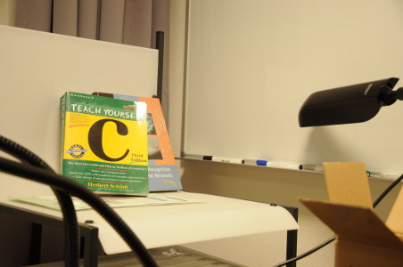
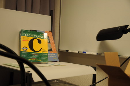
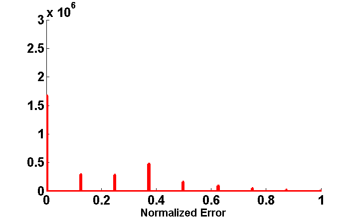
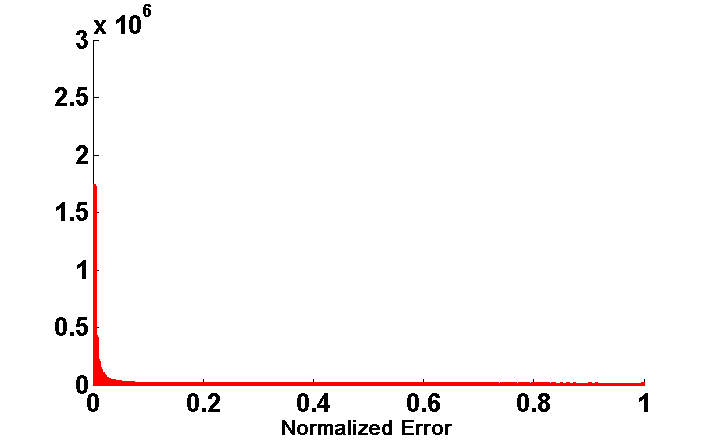
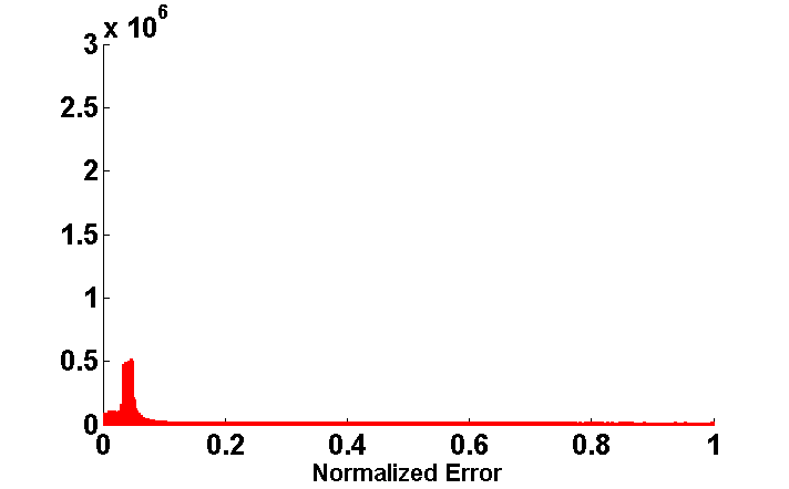
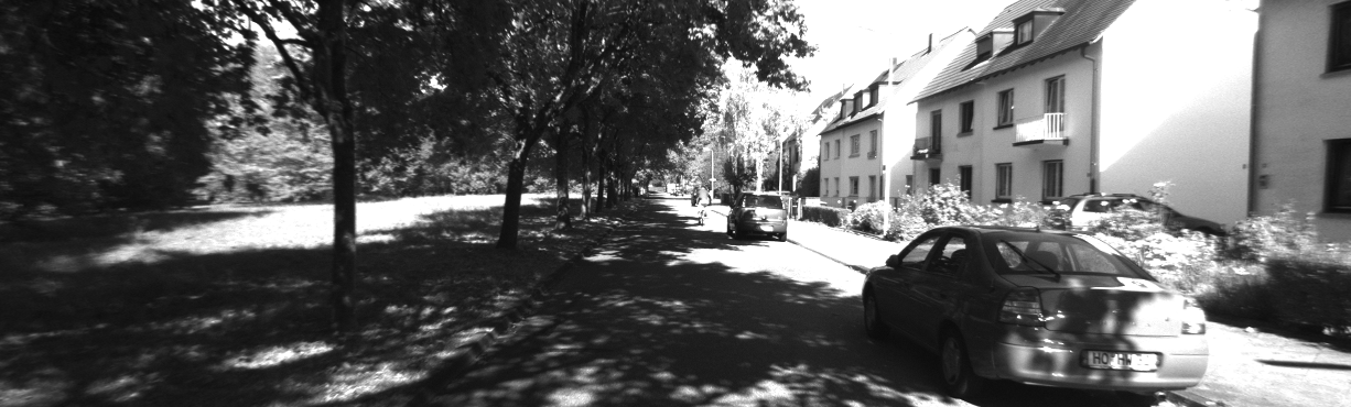
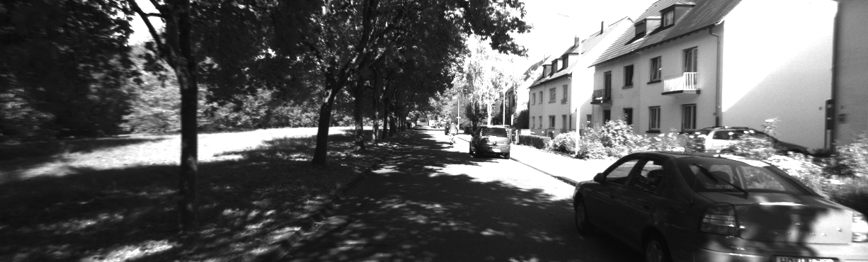
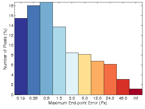
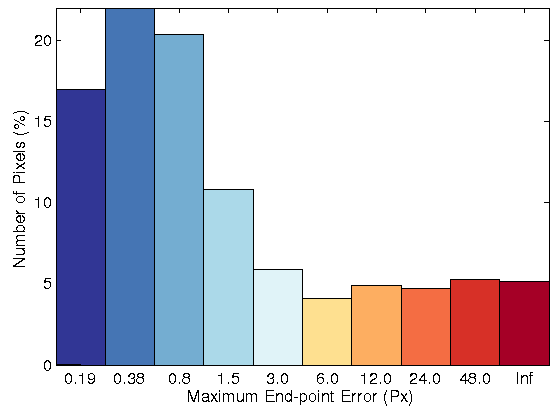
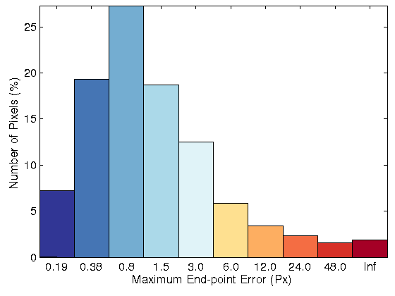
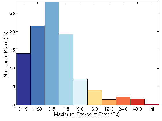
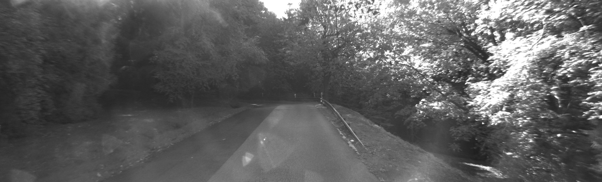
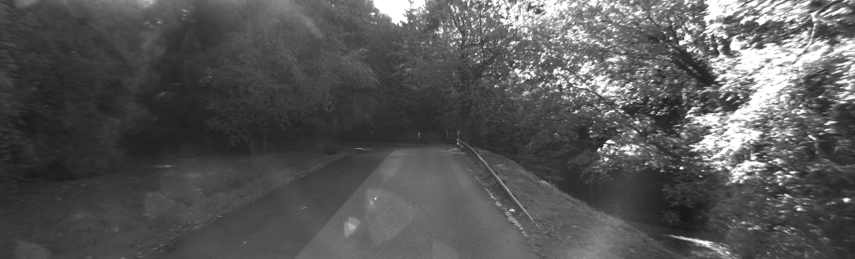
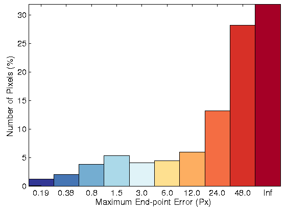
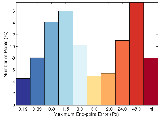
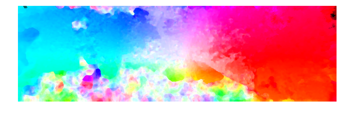
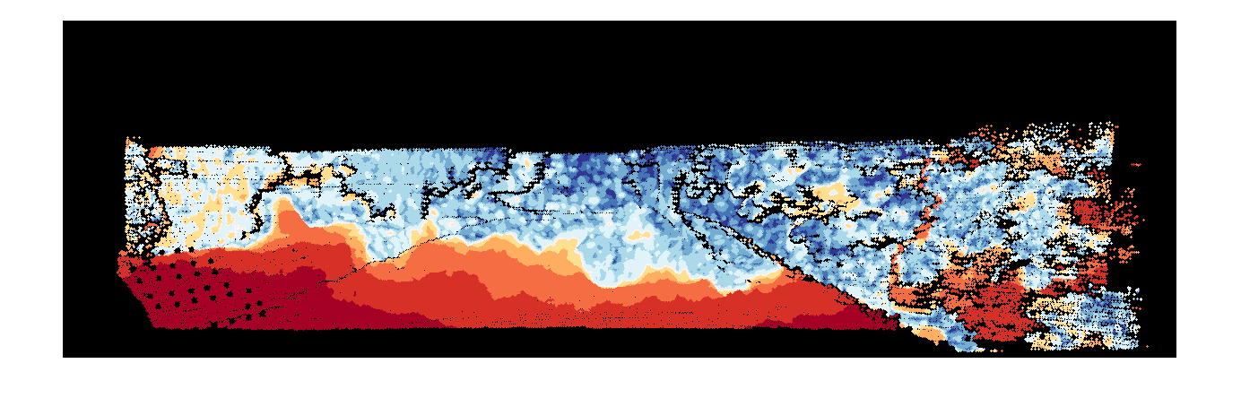
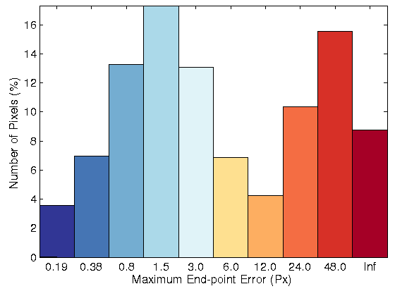
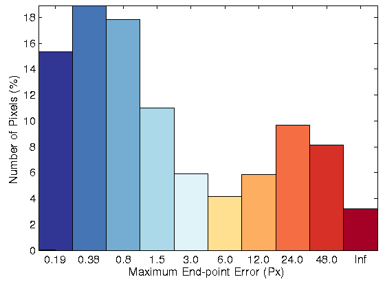
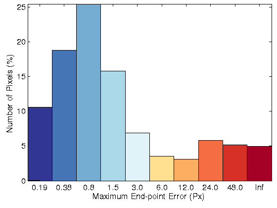
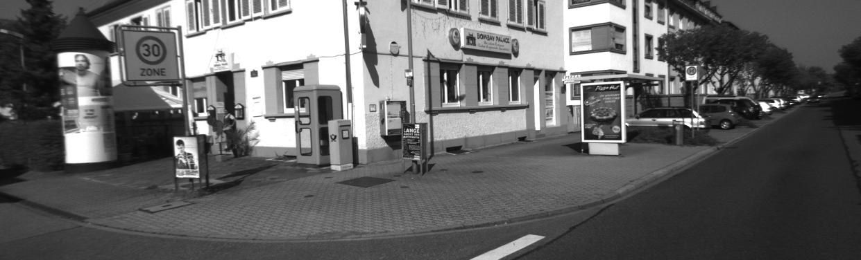
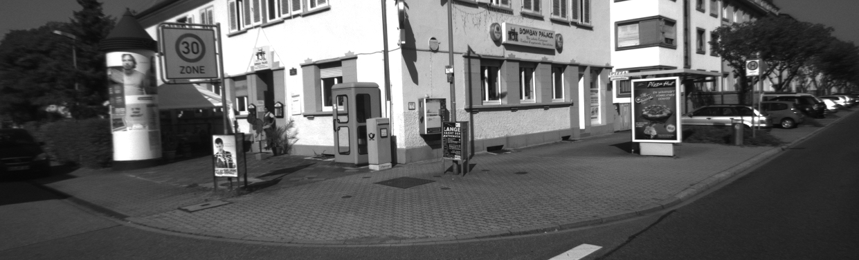
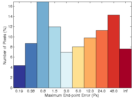
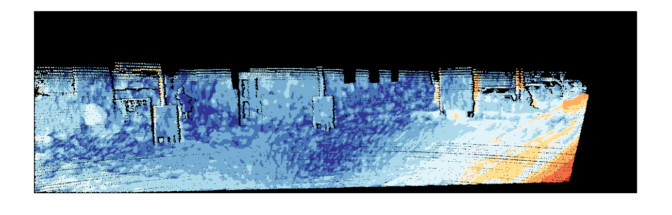
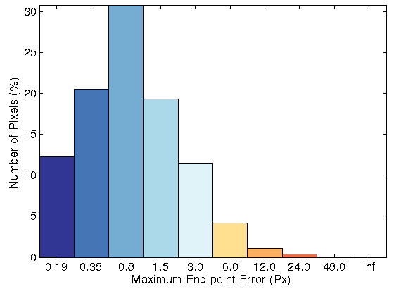
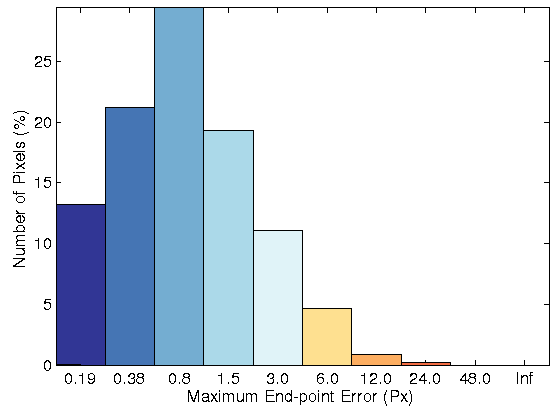
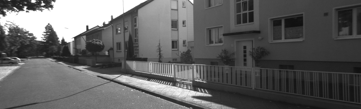
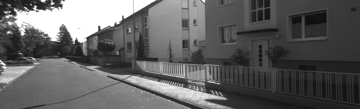
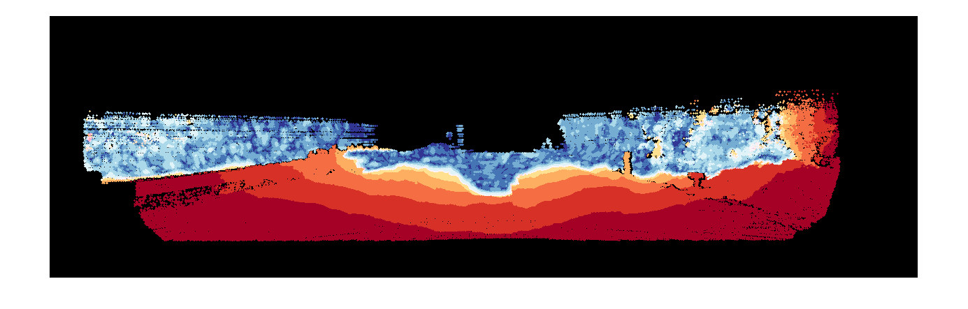
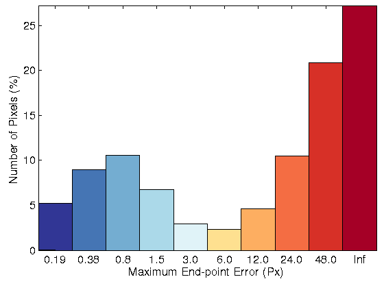
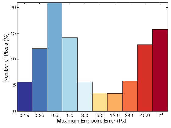
Figure 1 shows a real example that compares the performance of HOG, the census transform, the gradient constancy (GC) and the structure-texture decompensation ROF [6] using real images (2144 × 1424)for the same scene with different global illuminations. The comparison is performed by computing the histogram of normalized errors between
the same two features extracted from the pair of images. For the census transform, the error is computed based on the Hamming distance between the two descriptors (binary descriptors). In turn,
the error generated for HOG and ROF is the difference between the resulting features. In addition, the similarity between the pair of input images is obtained for the gradient constancy.
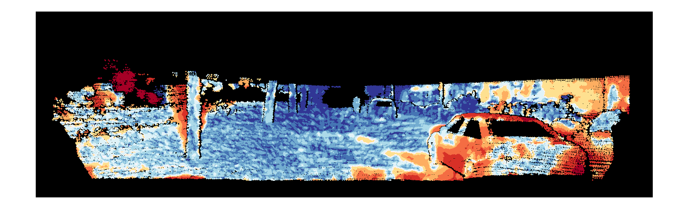
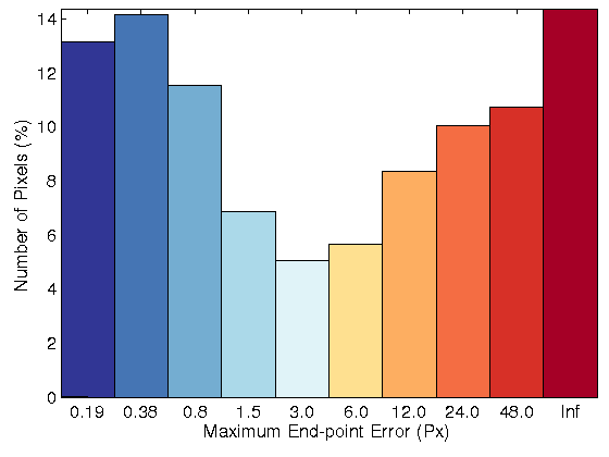
As shown in the figure, the gradient constancy yields the smallest average error(AE = 0.0146) among the different tested descriptors. However, HOG can detect the largest number of pixels
with zero error among them, as well as a good average error (AE = 0.0184). Thus, HOG is likely to be advantageous for motion estimation.
 |
 |
| (a) |
(b) |
 |
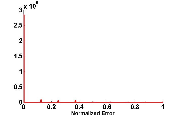 |
| (c) AE = 0.1595 |
(d) AE = 0.0184 |
 |
 |
| (e) AE = 0.0146 |
(f) AE = 0.0452 |
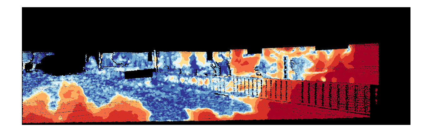
| Fig. 1: (a-b) Two original images. Error histograms for (c) CT, (d) HOG, (e) GC, and (f) ROF. |
Synthetic illumination
The variational optical flow model described has been tested with
different features descriptors by using sequence GROVE2 from the Middlebury
datasets with ground-truth by changing the illumination of the second frame as:
^{\gamma}\right))
where Ii and Io are the input and output frames, respectively, m > 0 is a
multiplicative factor, and γ > 0 is the gamma correction. The experiments are conducted in Matlab and the function uint8 is used for quantizing the values to
8-bit unsigned integer format.
 |
 |
| (a) |
(b) |
.png) |
 |
| (c) |
(d) |
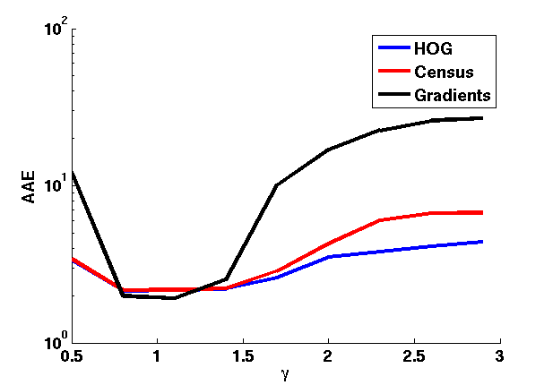
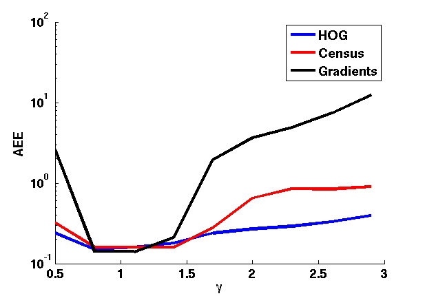
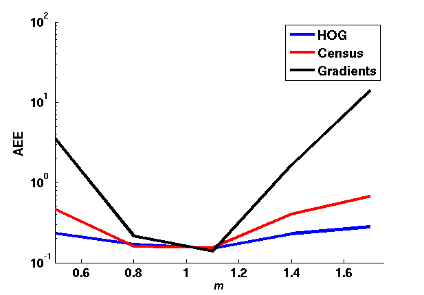
| Fig. 2: AEE and AAE for HOG, census transform and gradient constancy. Row 1: change of γ; row 2: change of m |
Figure 2 shows a qualitative comparison of the
average end-point error (AEE) and the average angular error (AAE) between
the flow fields obtained with HOG, the census transform, both determined in a
3 × 3 neighborhood, as well as the gradient constancy. The effects of different
values of m and γ have individually been assessed by varying γ while keeping
m = 1, and by changing m with γ = 1. As shown in figure 2, the gradient constancy is robust against small changes
of both γ and m. In turn, HOG shows a higher robustness against both small
and large changes of γ and m. In addition, the census transform yields adequate
values for both AEE and AAE.
Real illumination and large displacement test
Furthermore, the proposed variational optical flow method based on the HOG
descriptor is evaluated with eight real image sequences that include illumination
changes and large displacements, as well as low-textured areas, reflections and
specularities. Table 1 shows the AEE and bad pixels corresponding to four se-
quences with illumination changes and large displacements calculated for the
methods proposed in [1] , [2] , [3] ,
[4] , and [5] , in addition to the proposed
method based on HOG, the census transform and the gradient constancy.
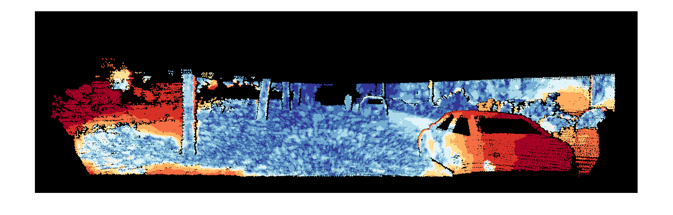
In another experiment, the estimated flow fields with HOG (3 × 3 and 5 × 5)
have visually been compared with the proposed optical flow method by using
the data term based on the brightness constancy assumption, as well as the
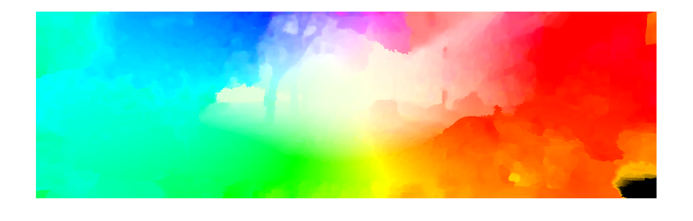
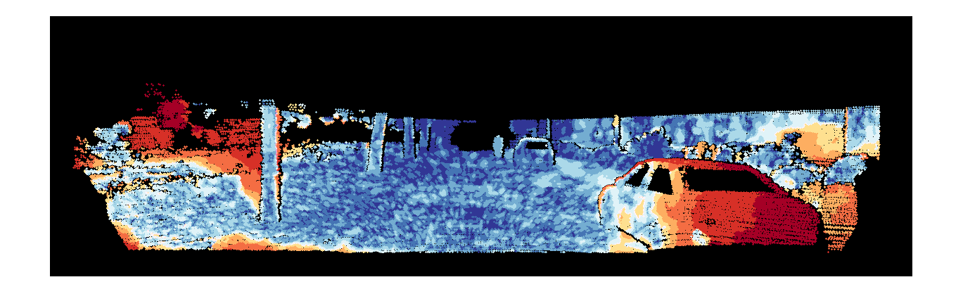
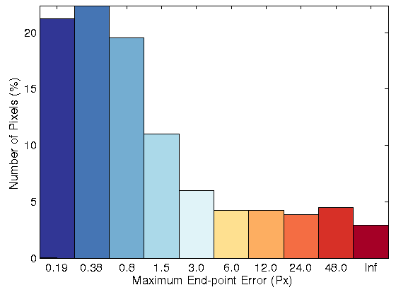
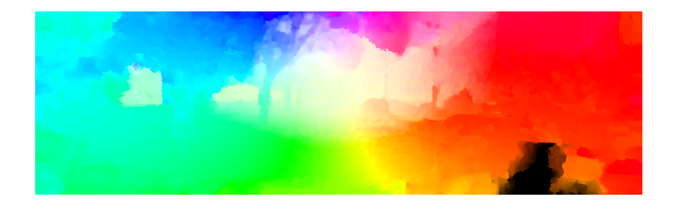
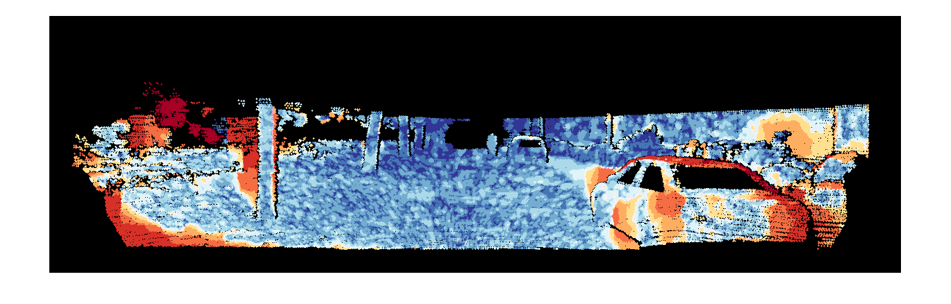
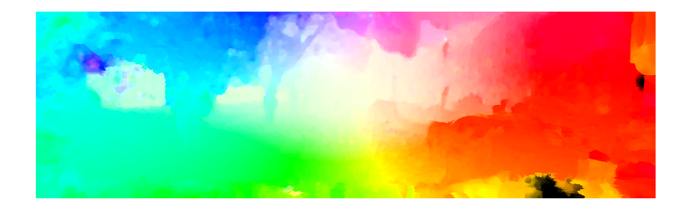
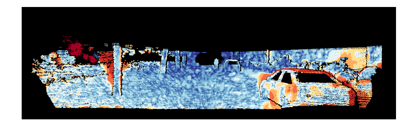
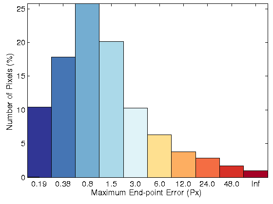
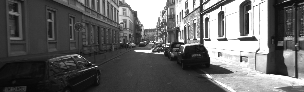
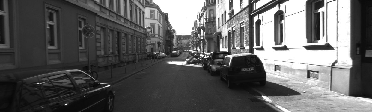
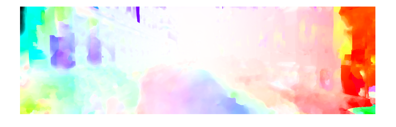
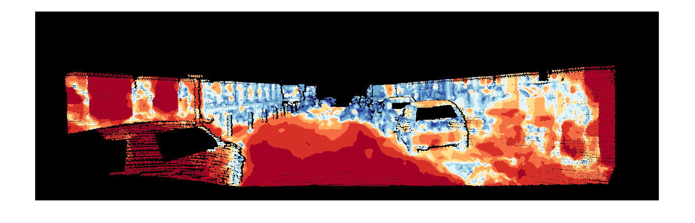
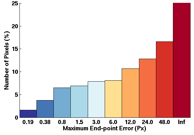
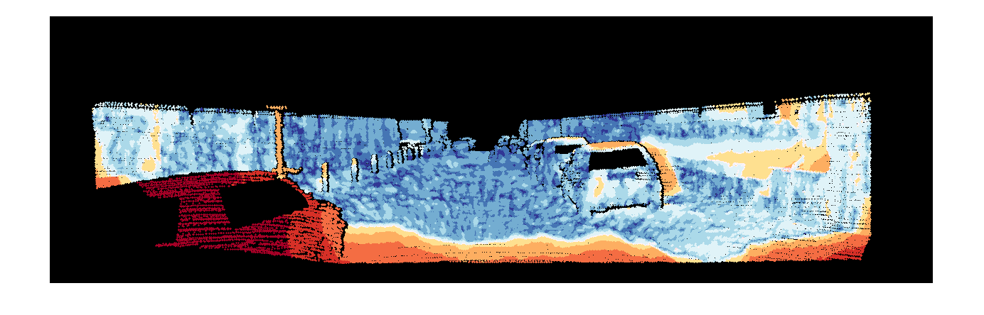
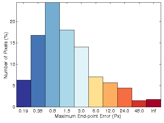
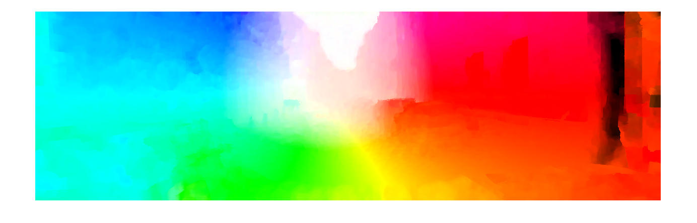
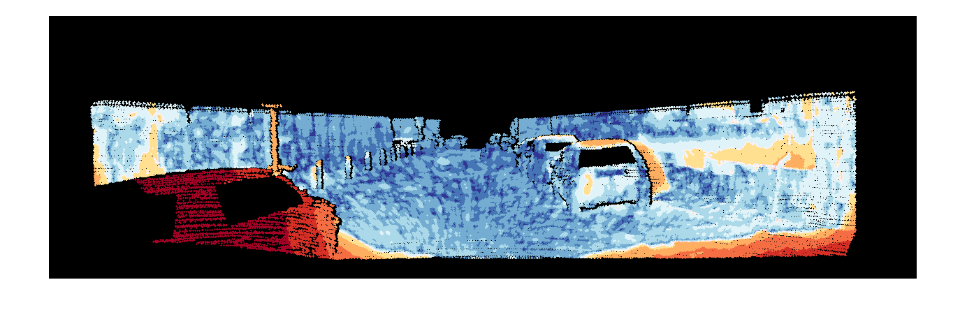
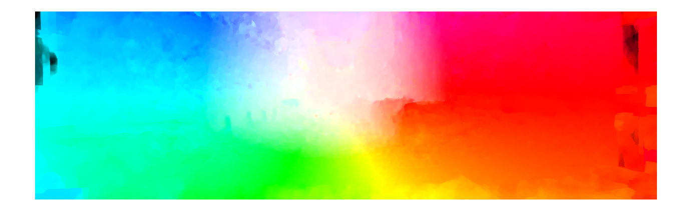
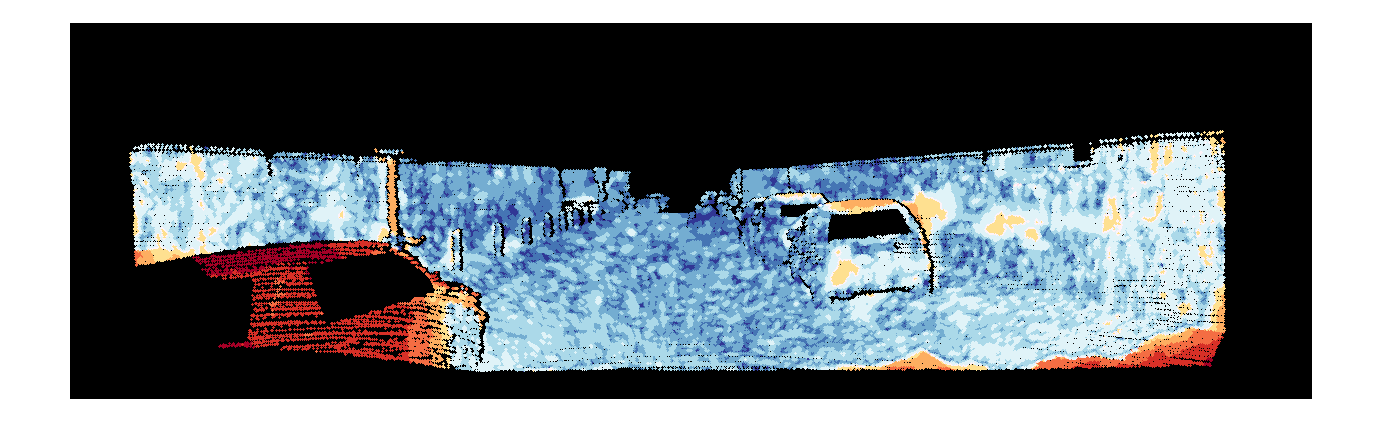
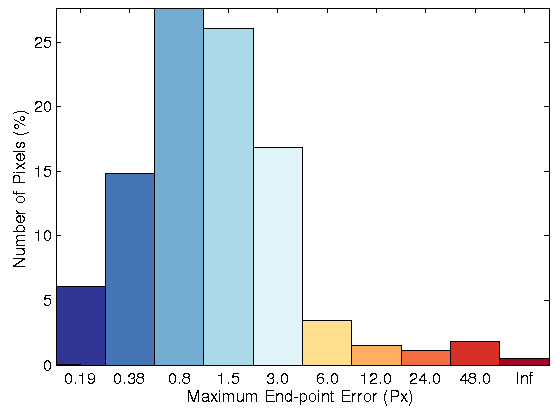
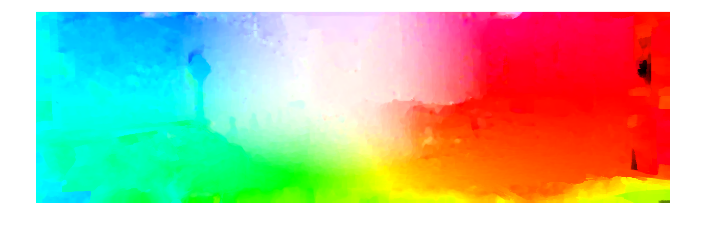
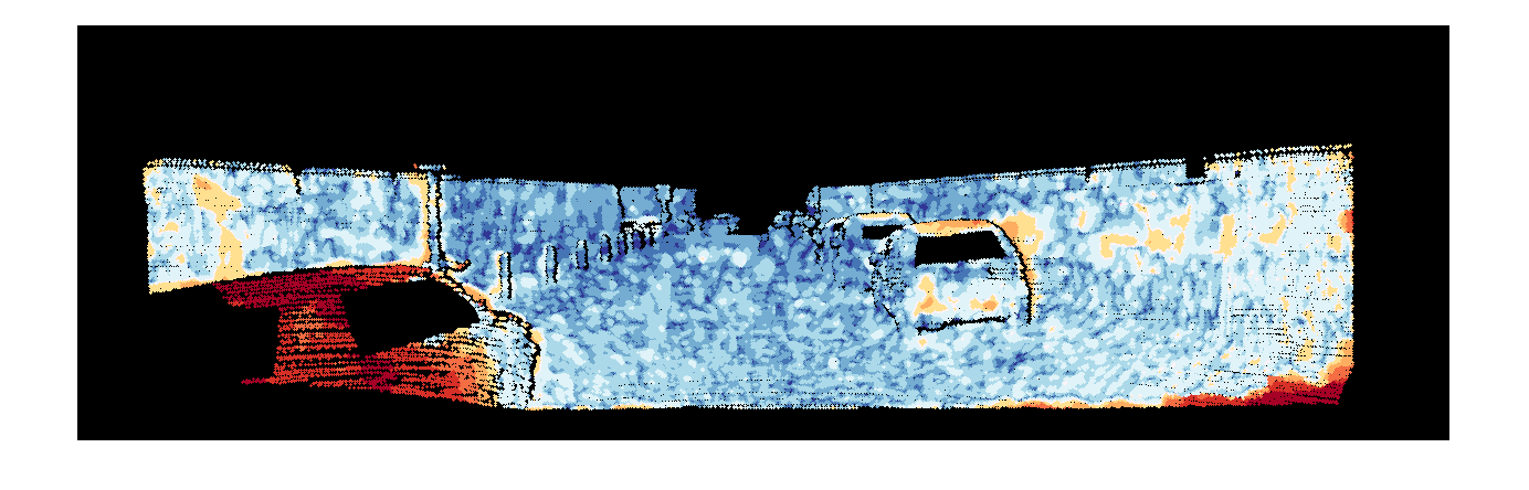
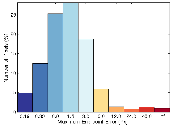
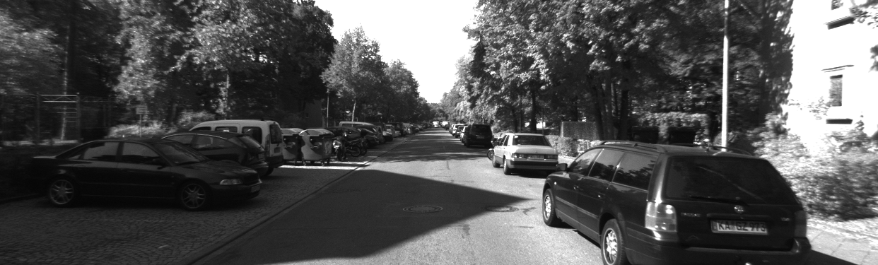
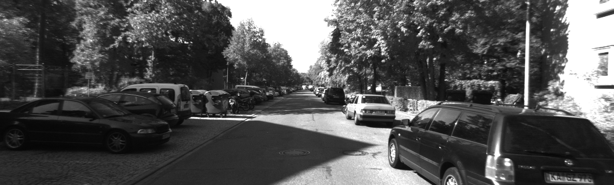
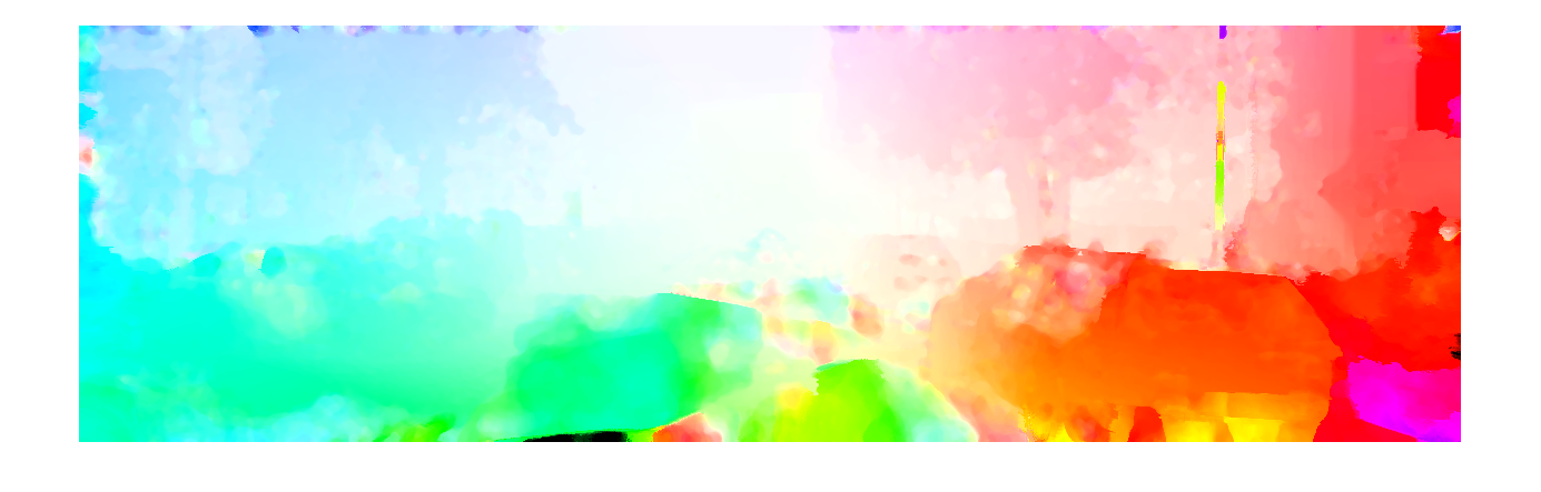
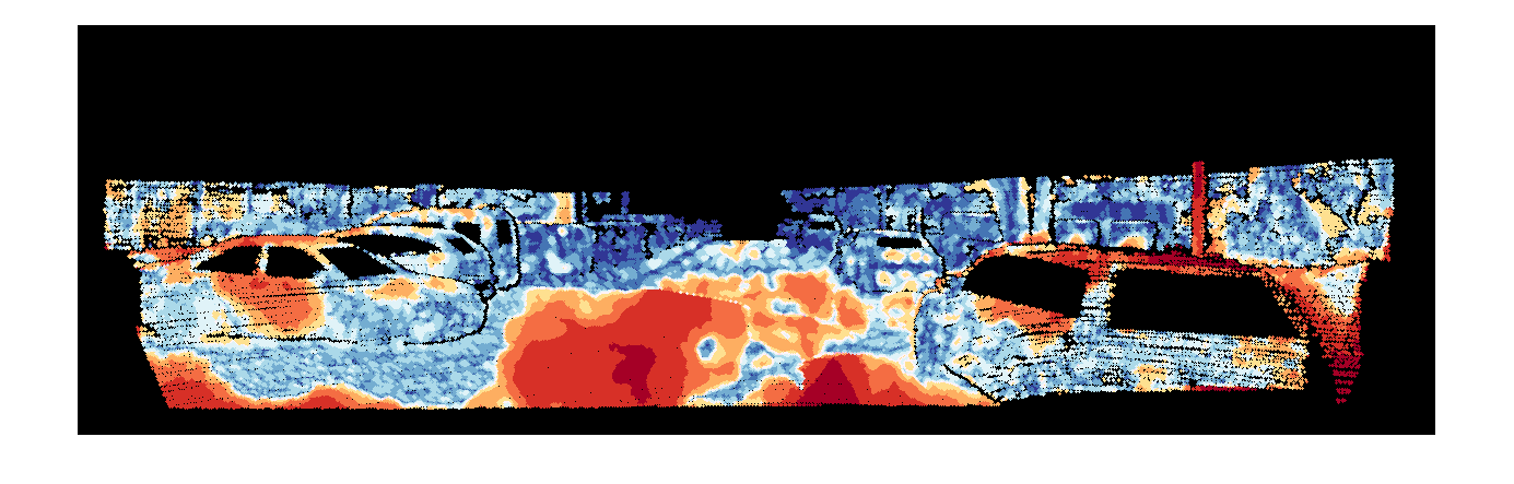
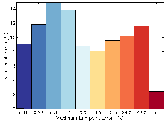
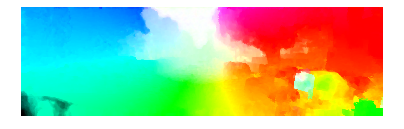
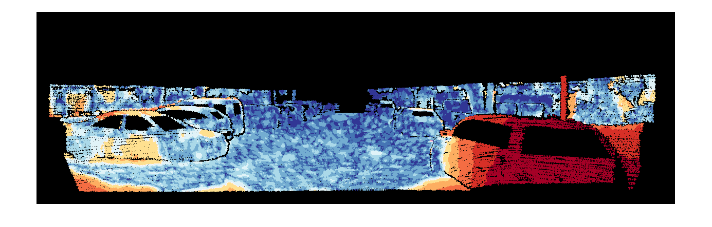
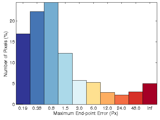
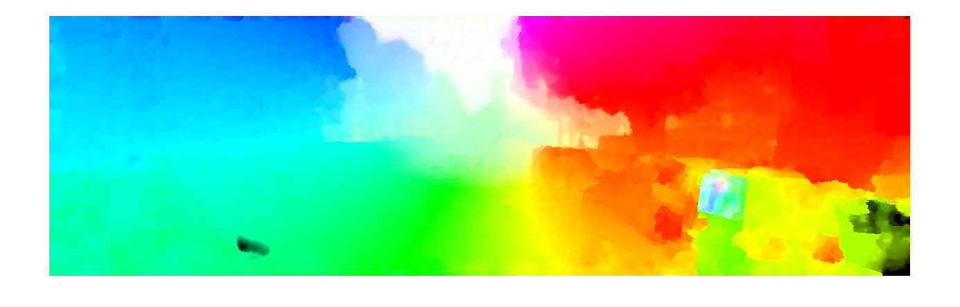
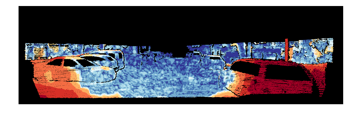
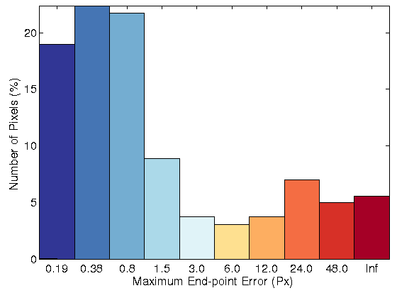
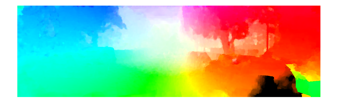
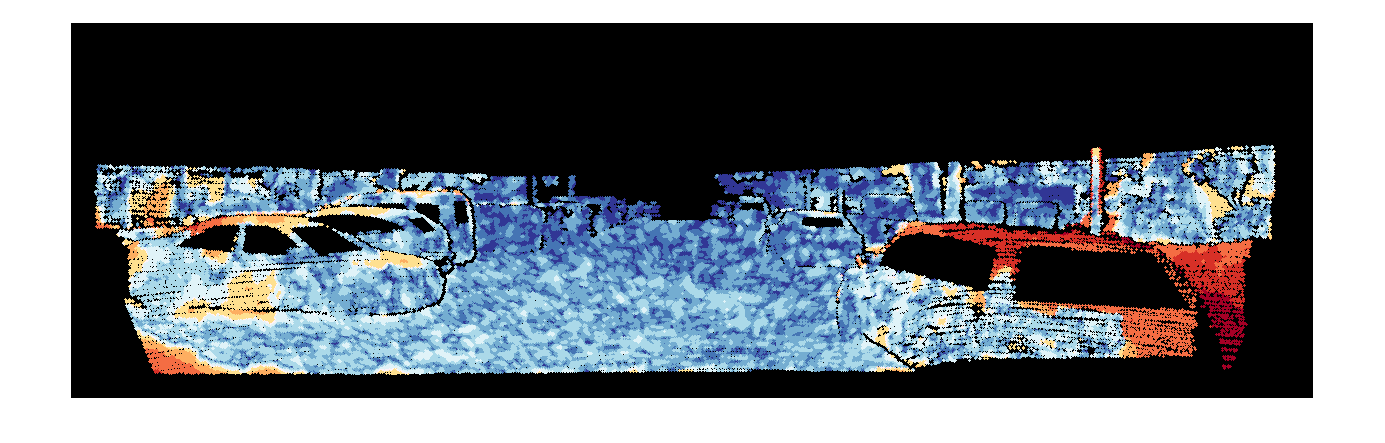
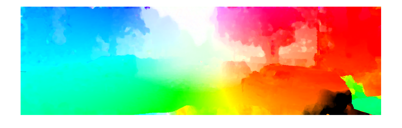
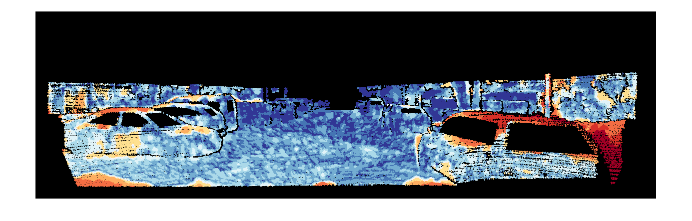
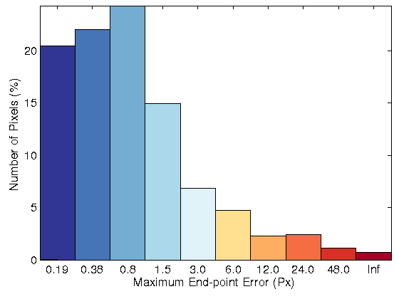
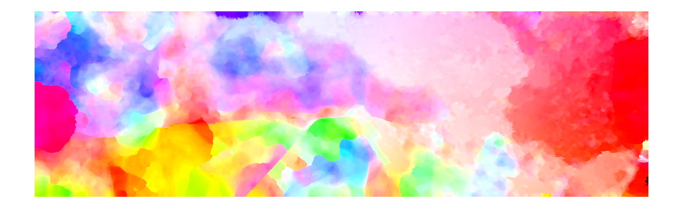
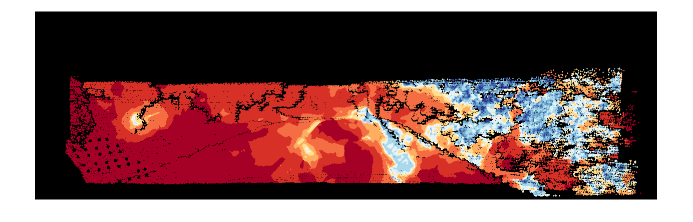
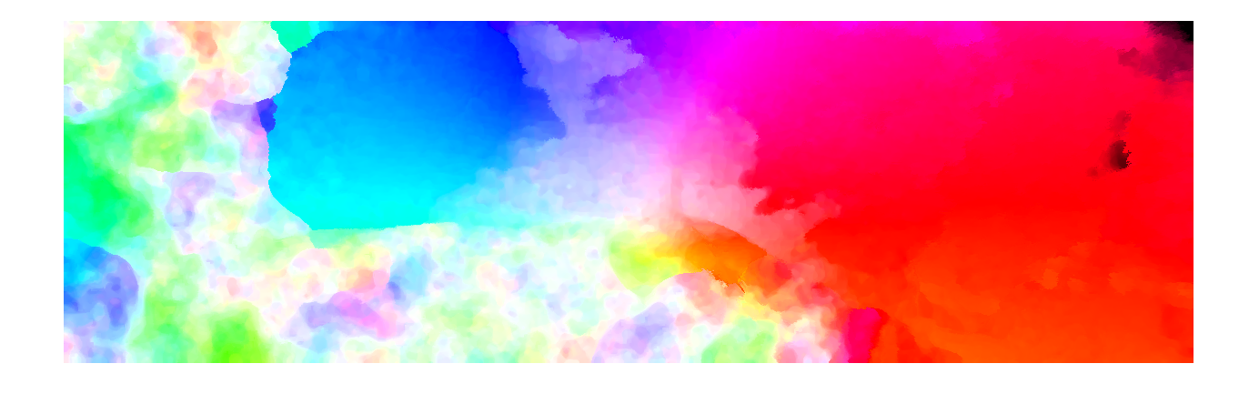
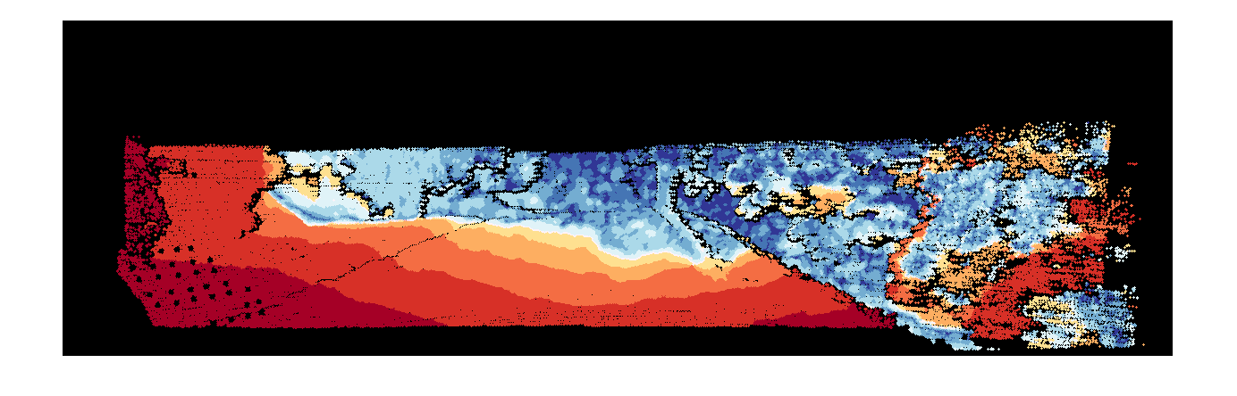
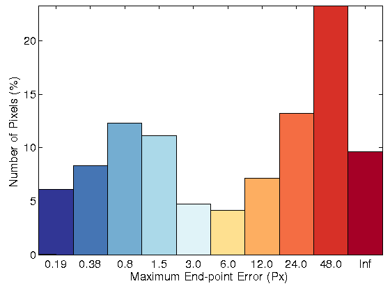
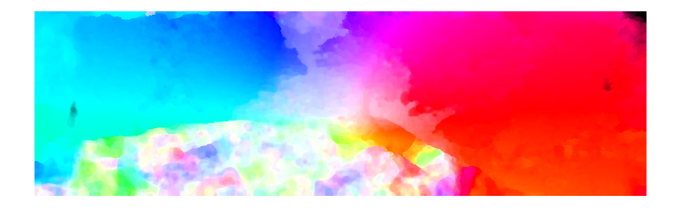
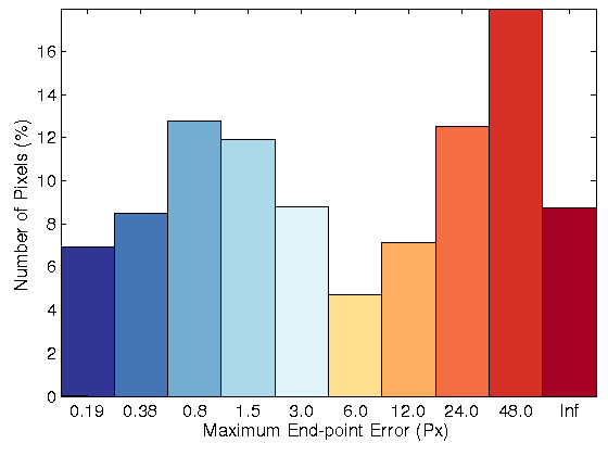
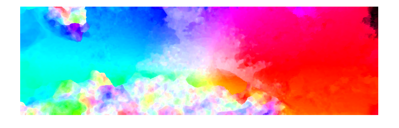
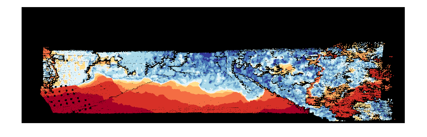
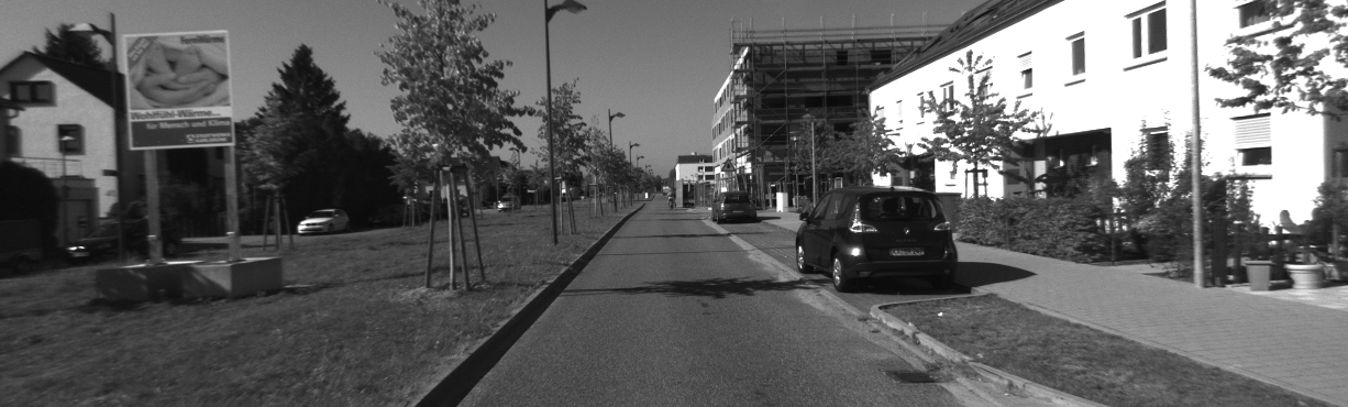
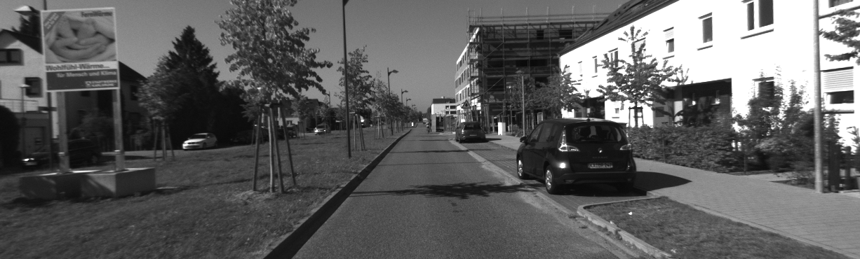
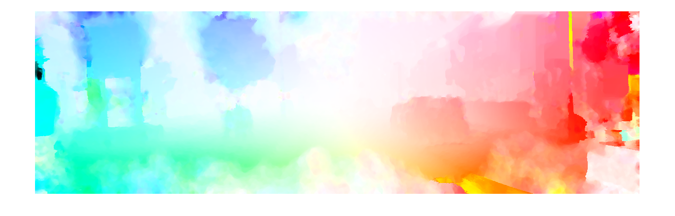
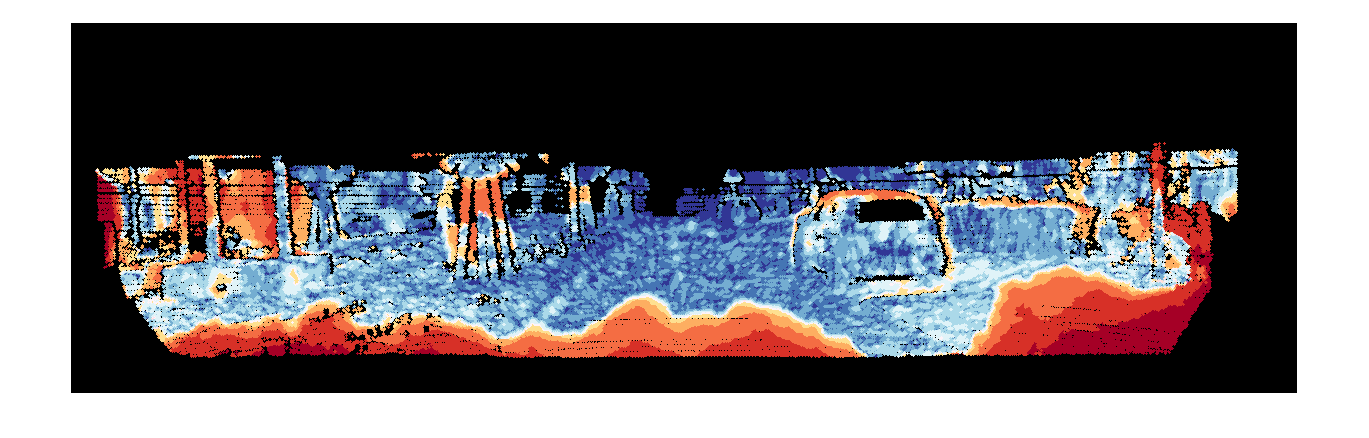
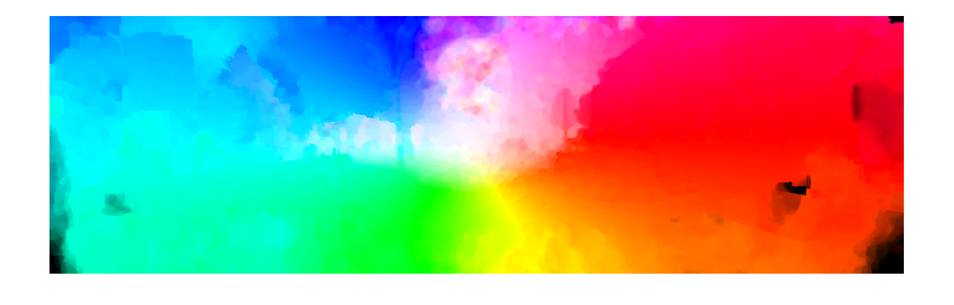
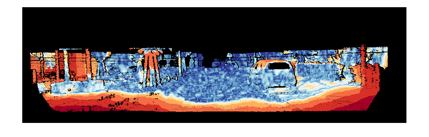
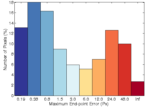
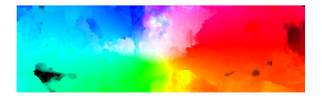
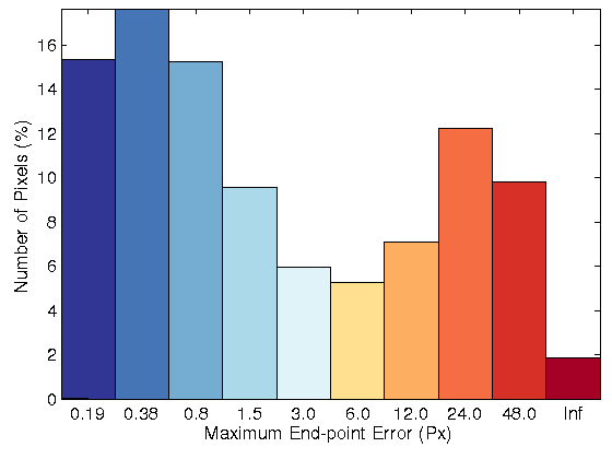
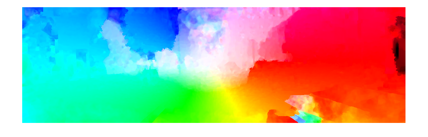
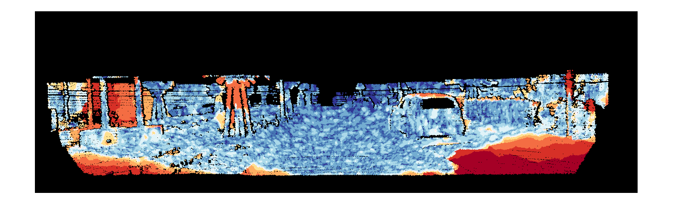
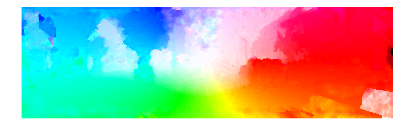
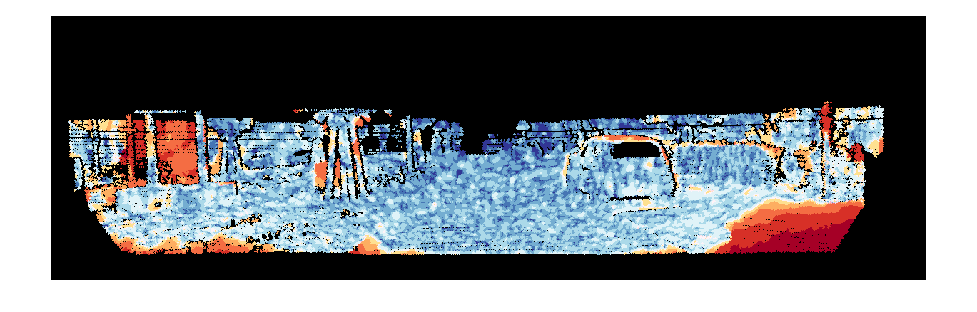
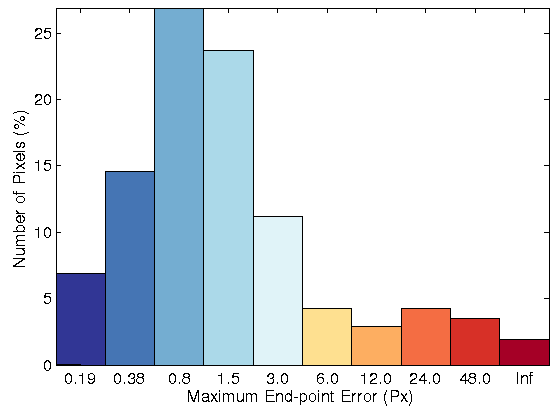
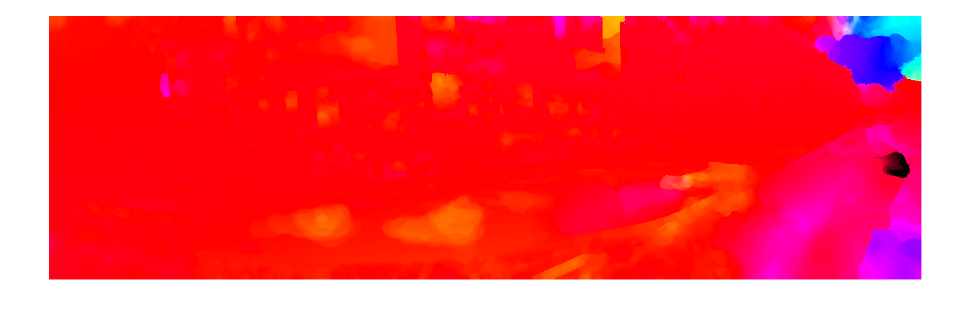
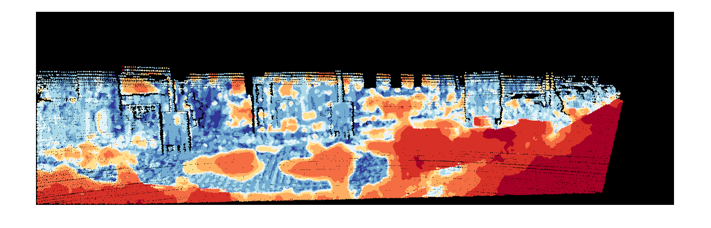
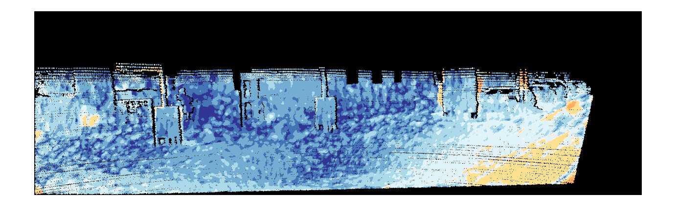
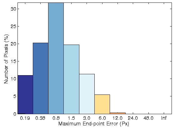
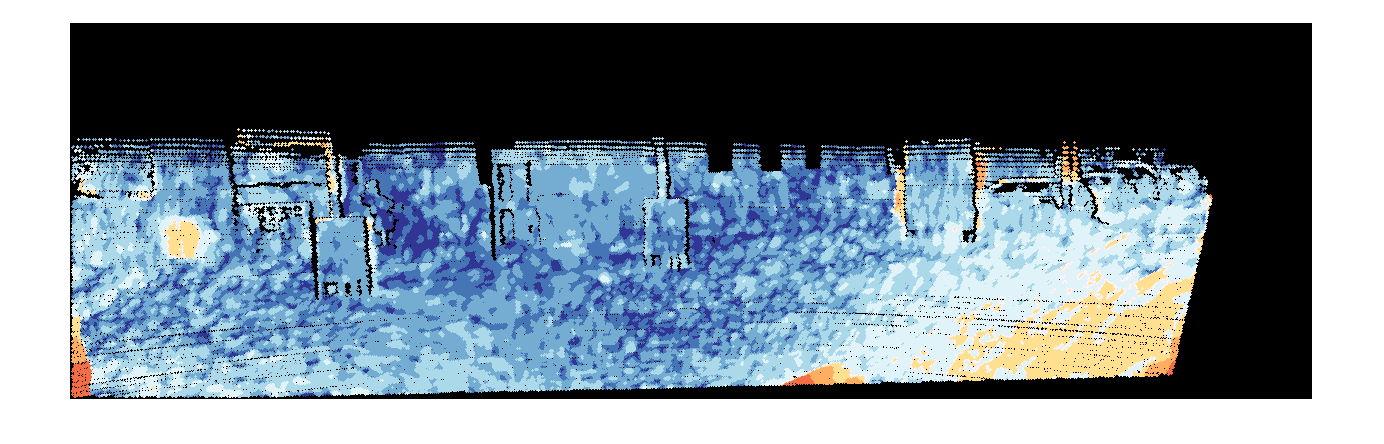
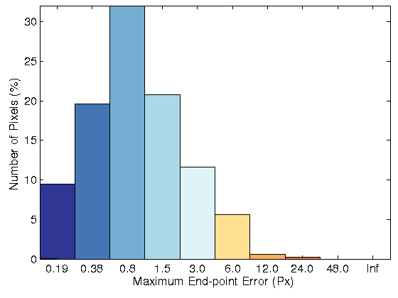
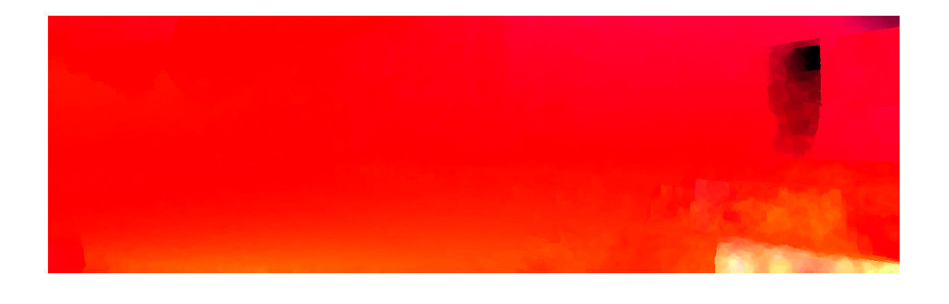
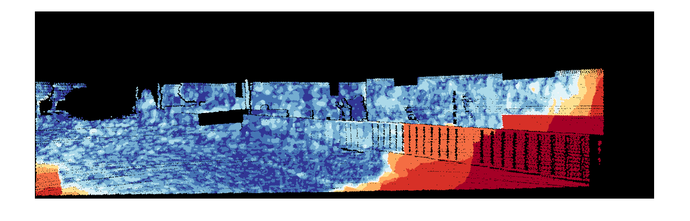
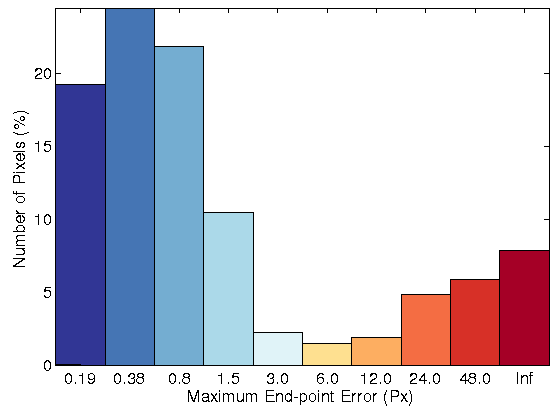
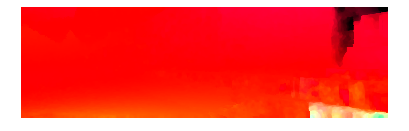
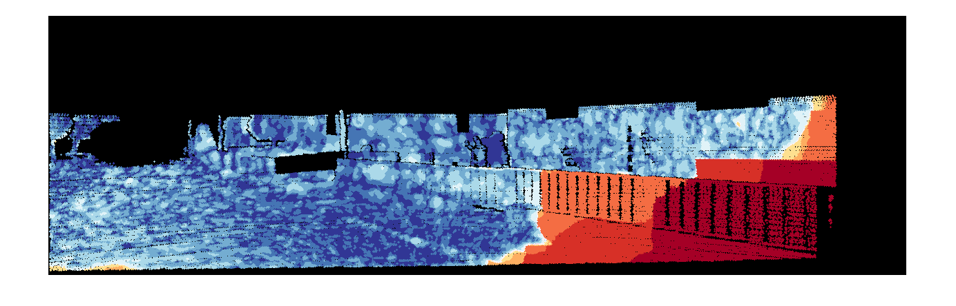
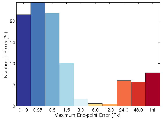
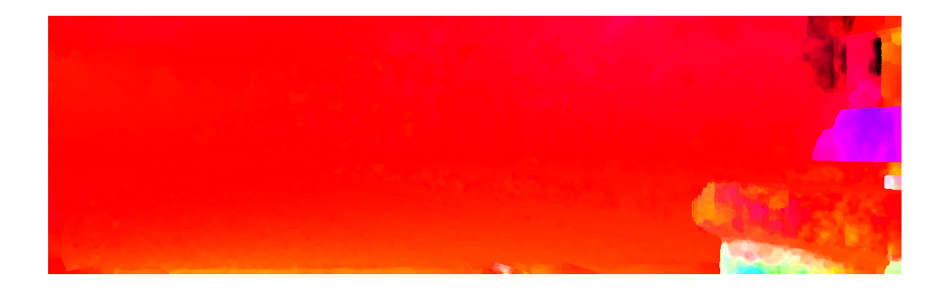
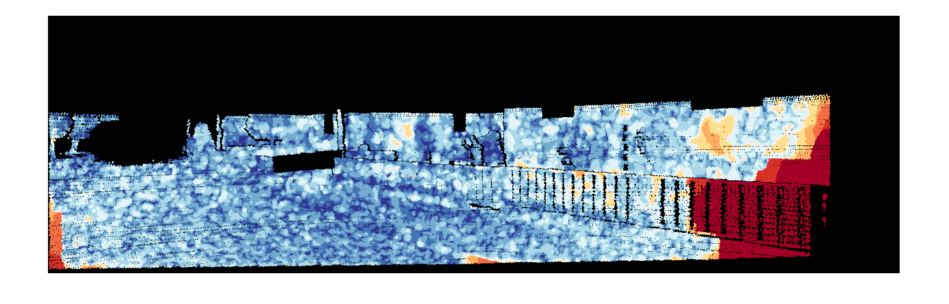
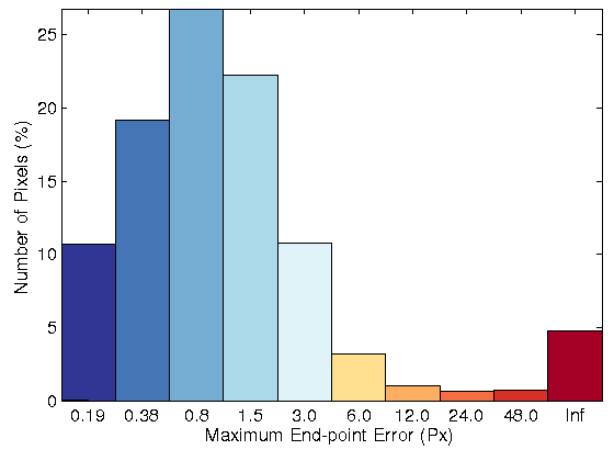
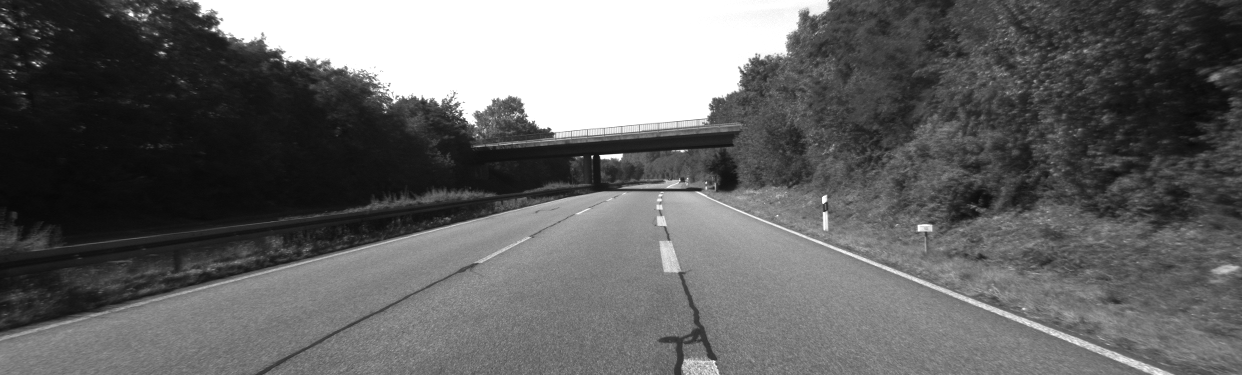
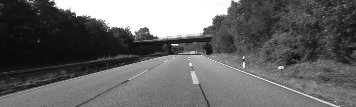
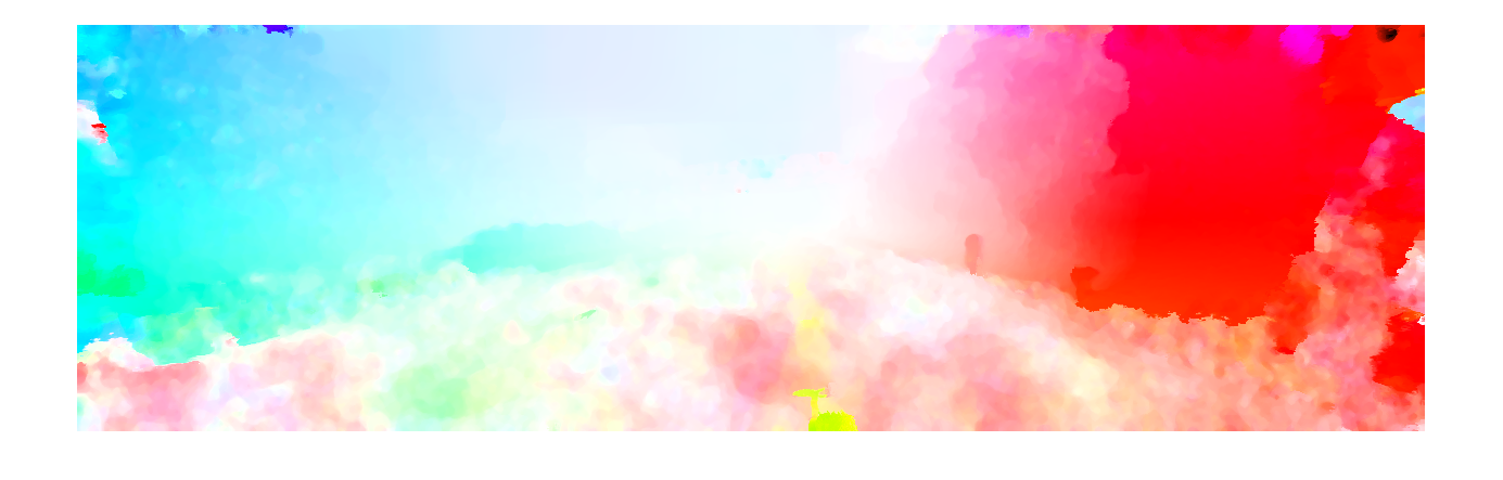
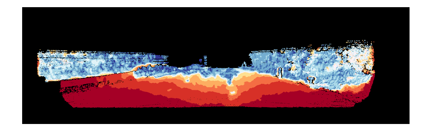
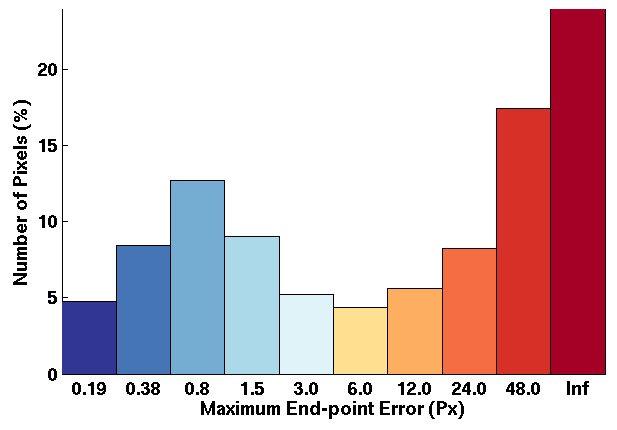
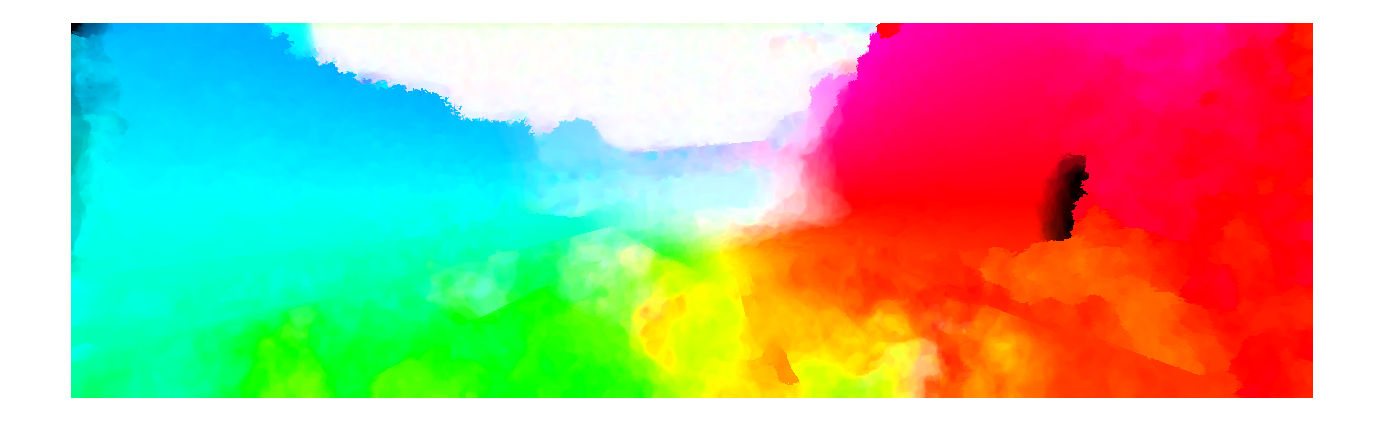
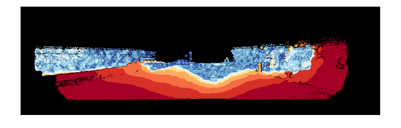
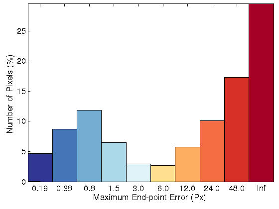
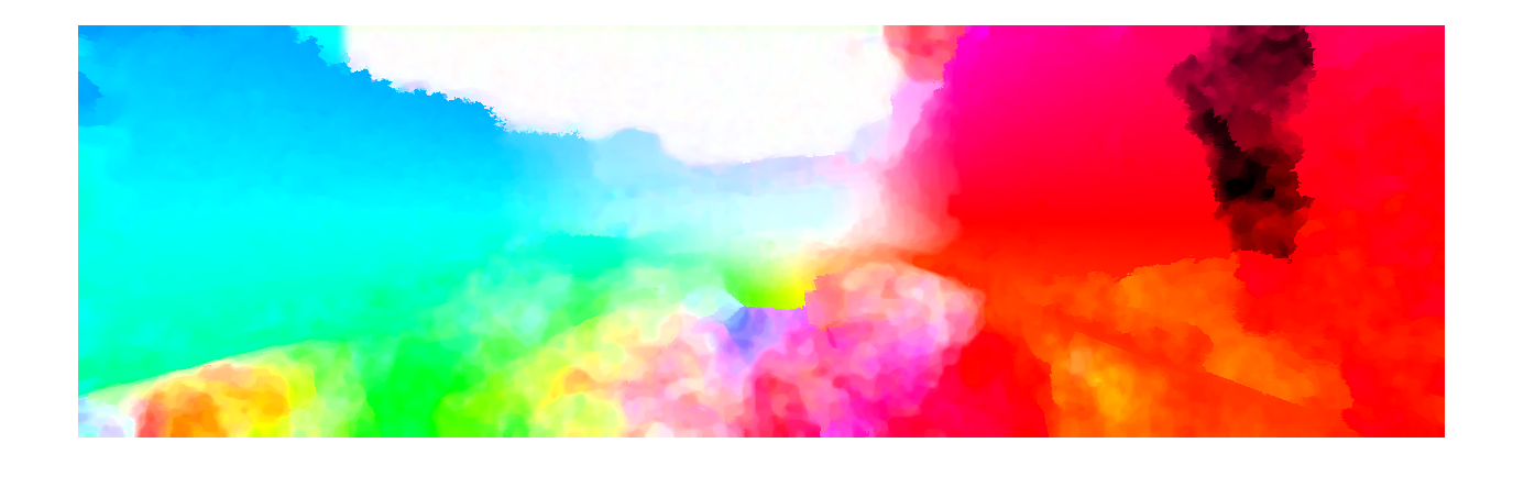
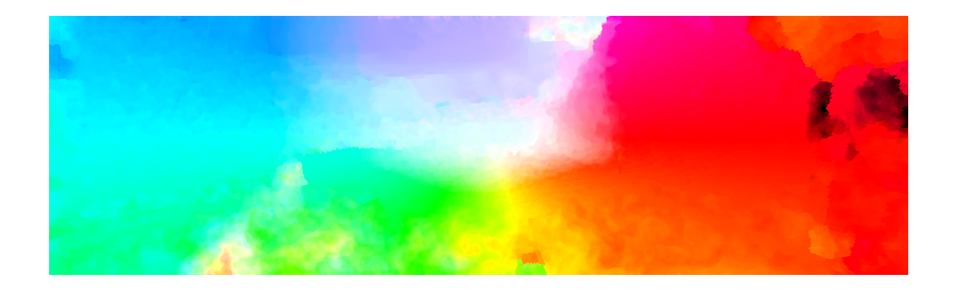
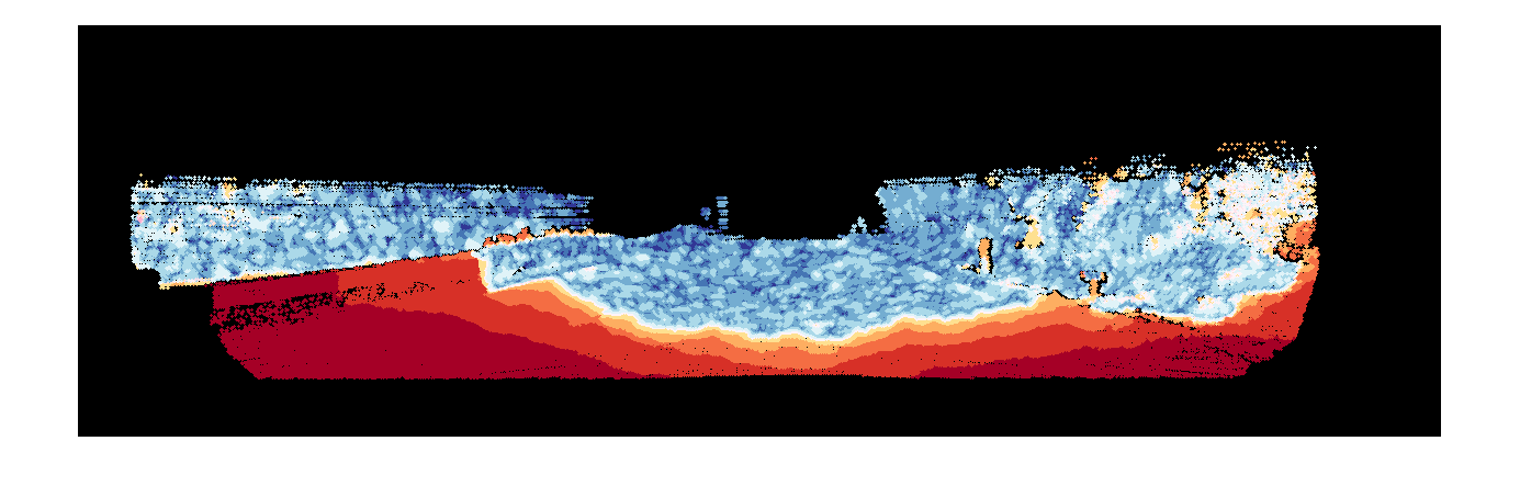
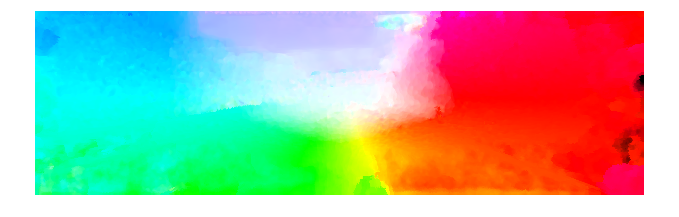
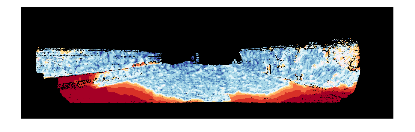
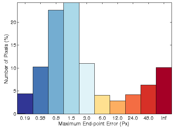
one based on the census transform. Figure 3 shows the estimated flow field for
sequence 15, which includes illumination changes, as well as the error images
and the error histograms. In addition, figure 4 shows the same information for
sequence 181, which includes large displacements. Among the evaluated approaches, the optical flow model based on HOG
yields the most accurate flow fields with respect to the state-of-the-art methods
for real images of KITTI datasets that include both illumination changes and
large displacements.
Table 1: Percentage of bad pixels and AEE for the state-of-the-art methods
and the proposed method with four sequences from KITTI datasets: sequences
11, 15, 44 and 74, which include illumination changes with the occluded points
ground truth.
| Method |
Seq 44 |
Seq 11 |
Seq 15 |
Seq 74 |
Average |
| HOG(3 x 3) |
21.45% (4.68) |
32.54% (9.04) |
22.30% (6.48) |
53.79% (20.03) |
32.52% |
| HOG(5 x 5) |
23.23% (5.22) |
29.92%(8.90) |
24.90% (7.64) |
52.74%(19.79) |
32.70% |
| Gradient Constancy |
29.25% (9.54) |
35.72%(10.91) |
26.41% (8.47) |
59.20% (23.07) |
37.64% |
| OFH 2011 [5] |
23.22% (5.11) |
37.26% (12.47) |
32.20% (9.06) |
62.90% (24.00) |
38.89% |
| Census(5 x 5) |
35.23% (12.74) |
33.93% (9.75) |
29.04% (8.70) |
57.57% (20.80) |
38.94% |
| Census(3 x 3) |
29.55% (10.22) |
37.54% (11.14) |
33.74% (9.11) |
57.43% (20.53) |
39.56% |
| SRB [3] |
26.58%(4.67) |
40.61% (13.76) |
32.85% (9.72) |
62.94% (24.27) |
40.74% |
| SRBF [3] |
31.83% (5.62) |
40.34% (13.96) |
35.13% (12.17) |
64.89% (24.64) |
43.05% |
| BW [1] |
32.44% (5.19) |
33.95% (8.50) |
47.70% (12.40) |
71.44% (25.15) |
46.38% |
| HS [2] |
42.96% (6.77) |
38.84% (10.72) |
58.08% (12.89) |
82.14% (28.75) |
55.50% |
| WPB [4] |
49.09% (9.20) |
49.99% (28.35) |
67.28% (28.36) |
88.67% (30.68) |
63.76% |
Table 2: Percentage of bad pixels and AEE for the state-of-the-art methods and
the proposed method with four sequences from KITTI datasets: sequences 11,
15, 44 and 74, which include illumination changes with the non-occluded points
ground truth.
| Method |
Seq 44 |
Seq 11 |
Seq 15 |
Seq 74 |
Average |
| HOG(3 x 3) |
9.98% (2.17) |
18.53% (3.78) |
8.40% (2.21) |
46.99%(14.20) |
20.98% |
| HOG(5 x 5) |
11.35% (2.26) |
15.54% ( 3.12) |
10.40%(2.41) |
45.76% (13.97) |
20.76% |
| Gradient Constancy |
16.78% (4.95) |
19.43%(4.01) |
11.97% (3.52) |
53.13% (16.38) |
25.33% |
| Census(5 x 5) |
24.30% (7.96) |
19.83% (5.06) |
15.03% (3.41) |
51.10%(15.14) |
27.57% |
| OFH [5] |
11.17% (2.44) |
24.32% (6.48) |
18.34% (3.63) |
57.40% (17.25) |
27.81% |
| SRB [3] |
14.66% (2.44) |
27.83% (6.43) |
18.93% (4.05) ) |
57.36% (17.36) |
29.69% |
| Census(3 x 3) |
18.26% (6.30) |
24.05% (7.28) |
20.30% (3.95) |
57.43%(17.53) |
30.01% |
| SRBF [3] |
20.98% (3.29) |
27.78% (6.73) |
21.66% (4.53) |
59.56% (17.52) |
32.49% |
| BW [1] |
22.38% (3.16) |
20.54% (3.62) |
36.85% (6.67) |
67.22% (18.49) |
36.75% |
| HS [2] |
34.18% (4.61) |
25.98% (6.79) |
49.57% (7.95) |
79.57% (21.55) |
47.32% |
| WPB [4] |
40.85% (5.88) |
39.25% (18.75) |
60.50% (17.63) |
87.02% (24.09) |
56.90% |
Sequence 11
 |
 |
| (a) |
(b) |
 |
 |
 |
Brightness Constrain |
 |
 |
 |
Census 3x3 |
 |
 |
 |
Census 5x5 |
 |
 |
 |
HOG 3x3 |
 |
 |
 |
HOG 5x5 |
| Fig. 1: (row 1) Two original images for sequence 15 of KITTI datasets. Resulting flow field, error image and error histogram for the proposed optical flow model
with: (row 2) brightness constancy, (row 3) 3 × 3 census transform, (row 4) 5 × 5 census transform, (row 5) 3 × 3 HOG, and (row 6) 5 × 5 HOG |
Sequence 15
 |
 |
| (a) |
(b) |
 |
 |
 |
Brightness Constrain |
 |
 |
 |
Census 3x3 |
 |
 |
 |
Census 5x5 |
 |
 |
 |
HOG 3x3 |
 |
 |
 |
HOG 5x5 |
| Fig. 2: (row 1) Two original images for sequence 15 of KITTI datasets. Resulting flow field, error image and error histogram for the proposed optical flow model
with: (row 2) brightness constancy, (row 3) 3 × 3 census transform, (row 4) 5 × 5 census transform, (row 5) 3 × 3 HOG, and (row 6) 5 × 5 HOG |
Sequence 44
 |
 |
| (a) |
(b) |
 |
 |
 |
Brightness Constrain |
 |
 |
 |
Census 3x3 |
 |
 |
 |
Census 5x5 |
 |
 |
 |
HOG 3x3 |
 |
 |
 |
HOG 5x5 |
| Fig. 3: (row 1) Two original images for sequence 15 of KITTI datasets. Resulting flow field, error image and error histogram for the proposed optical flow model
with: (row 2) brightness constancy, (row 3) 3 × 3 census transform, (row 4) 5 × 5 census transform, (row 5) 3 × 3 HOG, and (row 6) 5 × 5 HOG |
Sequence 74
 |
 |
| (a) |
(b) |
 |
 |
 |
Brightness Constrain |
 |
 |
 |
Census 3x3 |
 |
 |
 |
Census 5x5 |
 |
 |
 |
HOG 3x3 |
 |
 |
 |
HOG 5x5 |
| Fig. 4: (row 1) Two original images for sequence 15 of KITTI datasets. Resulting flow field, error image and error histogram for the proposed optical flow model
with: (row 2) brightness constancy, (row 3) 3 × 3 census transform, (row 4) 5 × 5 census transform, (row 5) 3 × 3 HOG, and (row 6) 5 × 5 HOG |
Table 3: Percentage of bad pixels and AEE for the state-of-the-art methods and
the proposed method with four sequences from KITTI datasets: sequences 117,
144, 147 and 181, which include large displacement with the occluded points
ground truth.
| Method |
Seq 147 |
Seq 117 |
Seq 144 |
Seq 181 |
Average |
| HOG(5 x 5) > |
14.04% (2.90) |
18.5% (12.27) |
31.64% (12.86) |
44.89% (33.72) |
27.27% |
| HOG(3 x 3) |
12.42% (2.87) |
24.49% (14.99) |
36.64% (14.40) |
55.58% (42.97) |
32.28% |
| OFH [5] |
15.04% (4.96) |
16.26% (4.33) |
42.04% (15.01) |
63.86% (50.52) |
34.30% |
| Gradient Constancy |
12.28% (3.93) |
17.70% (10.81) |
44.51% (18.67) |
67.63% (58.40) |
35.53% |
| SRB [3] |
14.59% (4.85) |
24.71% (9.74) |
50.67% (19.03) |
67.11% (47.70) |
39.27% |
| SRBF [3] |
14.79% (5.17) |
24.41% (9.92) |
50.66% (19.34) |
68.41% (48.81) |
39.57% |
| BW [1] |
16.98% (5.17) |
28.80% (7.86) |
46.98% (16.85) |
69.04% (45.27) |
40.45% |
| Census(5 x 5) |
13.98% (3.41) |
27.33% (15.23) |
47.68% (16.75) |
73.85% (58.59) |
40.71% |
| Census(3 x 3) |
14.76% (3.54) |
28.80% (15.20) |
48.97% (16.83) |
73.63% (58.58) |
41.54% |
| HS [2] |
24.84% (6.61) |
43.24% (15.32) |
51.89% (14.81) |
74.11% (49.28) |
48.52% |
| WPB [4] |
32.72% (8.10) |
46.80% (13.67) |
52.25% (17.94) |
76.00% (50.18) |
51.94% |
Table 4: Percentage of bad pixels and AEE for the state-of-the-art methods
and the proposed method with four sequences from KITTI datasets: sequences
117, 144, 147 and 181, which include large displacement with the non-occluded
points ground truth.
| Method |
Seq 147 |
Seq 117 |
Seq 144 |
Seq 181 |
Average |
| HOG(5 x 5) > |
6.41% (1.01) |
9.09% (5.42) |
16.82% (4.23) |
27.48% (11.97) |
14.95% |
| HOG(3 x 3) |
5.80% (0.92) |
17.04% (8.04) |
22.56% (6.85) |
41.44% (18.68) |
21.71% |
| OFH [5] |
8.03% (1.98) |
9.09% (2.17) |
29.62% (6.77) |
52.32% (23.46) |
24.76% |
| Gradient Constancy |
7.13% (1.25) |
9.70% (4.42) |
32.25% (8.26) |
57.21% (29.92) |
26.57% |
| SRB [3] |
7.55% (1.74) |
18.11% (5.28) |
39.55% (9.33) |
56.51% (22.88) |
30.43% |
| SRBF [3] |
7.69% (1.97) |
17.95% (5.29) |
39.64% (9.59) ) |
58.25% (23.78) |
30.88% |
| BW [1] |
10.07% (2.20) |
22.25% (4.23) |
35.01% (8.17) |
59.05% (22.58) |
31.60% |
| Census(5 x 5) |
6.78% (0.95) |
20.52% (9.82) |
36.29% (7.71) |
65.55% (31.26) |
32.29% |
| Census(3 x 3) |
6.63% (1.00) |
21.85% (9.59) |
37.49% (8.43) |
65.29% (31.92) |
32.82% |
| HS [2] |
18.52% (3.38) |
37.82% (9.77) |
41.30% (7.32) |
65.77% (23.40) |
40.85% |
| WPB [4] |
25.92% (4.43) |
41.23% (9.18) |
41.53% (8.94) |
68.27% (25.96) |
44.24% |
Sequence 144
 |
 |
| (a) |
(b) |
 |
 |
 |
Brightness Constrain |
 |
 |
 |
Census 3x3 |
 |
 |
 |
Census 5x5 |
 |
 |
 |
HOG 3x3 |
 |
 |
 |
HOG 5x5 |
| Fig. 5: (row 1) Two original images for sequence 15 of KITTI datasets. Resulting flow field, error image and error histogram for the proposed optical flow model
with: (row 2) brightness constancy, (row 3) 3 × 3 census transform, (row 4) 5 × 5 census transform, (row 5) 3 × 3 HOG, and (row 6) 5 × 5 HOG |
Sequence 147
 |
 |
| (a) |
(b) |
 |
 |
 |
Brightness Constrain |
 |
 |
 |
Census 3x3 |
 |
 |
 |
Census 5x5 |
 |
 |
 |
HOG 3x3 |
 |
 |
 |
HOG 5x5 |
| Fig. 6: (row 1) Two original images for sequence 15 of KITTI datasets. Resulting flow field, error image and error histogram for the proposed optical flow model
with: (row 2) brightness constancy, (row 3) 3 × 3 census transform, (row 4) 5 × 5 census transform, (row 5) 3 × 3 HOG, and (row 6) 5 × 5 HOG |
Sequence 117
 |
 |
| (a) |
(b) |
 |
 |
 |
Brightness Constrain |
 |
 |
 |
Census 3x3 |
 |
 |
 |
Census 5x5 |
 |
 |
 |
HOG 3x3 |
 |
 |
 |
HOG 5x5 |
| Fig. 7: (row 1) Two original images for sequence 15 of KITTI datasets. Resulting flow field, error image and error histogram for the proposed optical flow model
with: (row 2) brightness constancy, (row 3) 3 × 3 census transform, (row 4) 5 × 5 census transform, (row 5) 3 × 3 HOG, and (row 6) 5 × 5 HOG |
Sequence 181
 |
 |
| (a) |
(b) |
 |
 |
 |
Brightness Constrain |
 |
 |
 |
Census 3x3 |
 |
 |
 |
Census 5x5 |
 |
 |
 |
HOG 3x3 |
 |
 |
 |
HOG 5x5 |
| Fig. 8: (row 1) Two original images for sequence 15 of KITTI datasets. Resulting flow field, error image and error histogram for the proposed optical flow model
with: (row 2) brightness constancy, (row 3) 3 × 3 census transform, (row 4) 5 × 5 census transform, (row 5) 3 × 3 HOG, and (row 6) 5 × 5 HOG |
KITTI dataset
The proposed variational optical flow method tested upon the widely used KITTI dataset optical flow. According to the KITTI
(April 2013), the results of the proposed model with HOG (TVL1-HOG) have been evaluated, and it has been ranked in the 7 position out of 32 current state-of-the-art optical flow algorithms. The KITTI benchmark considers the bad flow vectors at all pixels that are above a spatial distance of 3 pixels from the ground truth. (TVL1-
HOG) has average of 8.31% bad pixels, in turn the baseline methods [7] and [3] have 30.75% and 24.64%, respectively.
| Rank |
Method |
Out-Noc |
Out-All |
Avg-Noc |
Avg-All |
| 1 |
PR-Sf+E |
4.08 % |
7.79 % |
0.9 px |
1.7 px |
| 2 |
PCBP-Flow |
4.08 % |
8.70 % |
0.9 px |
2.2 px |
| 3 |
MotionSLIC |
4.36 % |
10.91 % |
1.0 px |
2.7 px |
| 4 |
PR-Sceneflow |
4.48 % |
8.98 % |
1.3 px |
3.3 px |
| 5 |
TGV2ADCSIFT |
6.55 % |
15.35 % |
1.6 px |
4.5 px |
| 6 |
Data-Flow |
8.22 % |
15.78 % |
2.3 px |
5.7 px |
| 7 |
TVL1-HOG |
8.31 % |
19.21 % |
2.0 px |
6.1 px |
| 8 |
MLDP-OF |
8.91 % |
18.95 % |
2.5 px |
6.7 px |
| 9 |
CRTflow |
9.71 % |
18.88 % |
2.7 px |
6.5 px |
| 10 |
C++ |
10.16 % |
20.29 % |
2.6 px |
7.1 px |
References
| 1. |
A. Bruhn and J. Weickert. Towards ultimate motion estimation: Combining highest accuracy with real-time performance. In ICCV, pages 749-755, 2005. |
| 2. |
B. Horn and B. Schunk. Determining optical flow. In Artificial Intelligence, vol. 17, pages 185-203, 1981. |
| 3. |
D. Sun, S. Roth, and M.J. Black. Secrets of optical flow estimation and their principles. In CVPR, pages 24322439. IEEE, 2010. |
| 4. |
M. Werlberger, T. Pock, and H. Bischof. Motion estimation with non-local total variation regularization. In CVPR, pages 2464-2471.IEEE, 2010. |
| 5. |
H. Zimmer, A. Bruhn, and J. Weickert. Optic flow in harmony. In IJCV, vol. 93(3): pages 368-388, 2011. |
| 6. |
Rudin, L.I., Osher, S.J., Fatemi, E.: Nonlinear total variation based noise removal algorithms. In Physica D, vol. 60, pages 259-268, 1992 |
| 7. |
C. Zach, T. Pock, H. Bischof, A duality based approach for realtime tv- l1 optical flow. In DAGM. pages 214-223, 2007 |
| 8. |
H. Rashwan, M. Mohamed, M. Garcia, B. Mertsching, and D. Puig.
Illumination Robust Optical Flow Model Based on Histogram of Oriented Gradients.
In: German Conference on Pattern Recognition, Springer Berlin Heidelberg, 2013, Lecture Notes in Computer Science. |
Contact
Do you have any questions or comments? Please contact:
|