Abstract
Most variational optical flow methods are based on
the well-known brightness constancy assumption or high-order
constancy assumptions in order to implement the data term in
the optimization energy function. Unfortunately, any variation
in the lighting within the scene violates the brightness constancy
constraint; in turn, the gradient constancy assumption does
not work properly with large illumination changes. This paper
proposes an illumination-robust constancy based on a robust
texture descriptor rather than the brightness constancy. Thus,
the similarity function used as a data term was obtained from
extracting texture features through the local directional pattern
descriptor for two consecutive frames within the duality total
variational optical flow algorithm. In addition, a weighted non-
local term that depends on both the color similarity and the
occlusion state of pixels is integrated during the optimization
process in order to increase the accuracy of the resulting flow
field. Experimental results show a qualitative comparison with the
proposed approach and yield state-of-the-art results on KITTI
datasets
Experimental Results
The proposed variational optical flow model was tested with different feature descriptors using sequence GROVE2 from the Middlebury datasets with ground-truth
Middlebury by changing the illumination of the second frame depending on:
^{\gamma}\right))
where Ii and Io are the input and output frames, respectively, m > 0 is a
multiplicative factor, a>0 is an additive change factor and γ > 0 is the gamma correction.
The experiments are conducted in Matlab and the function uint8 is used for quantizing the values to
8-bit unsigned integer format.
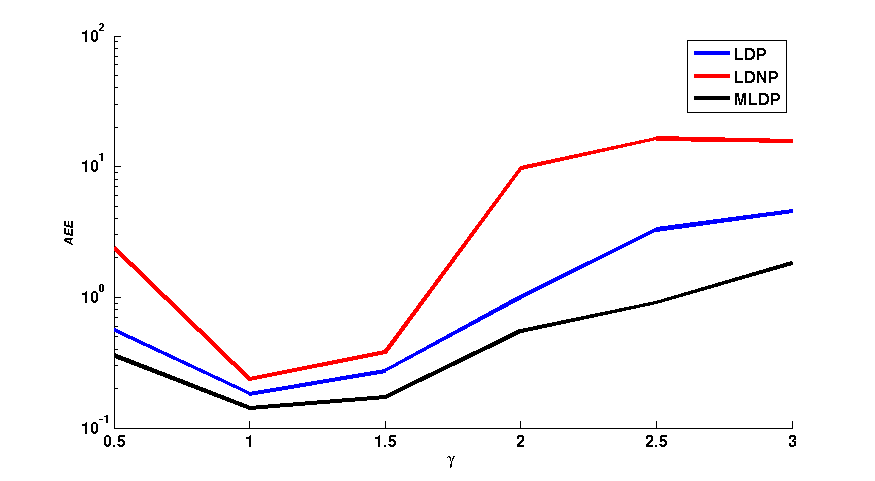
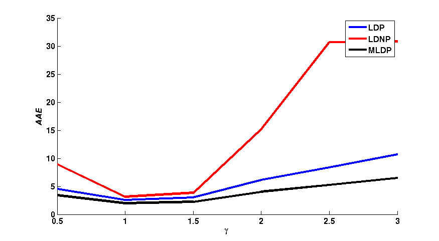
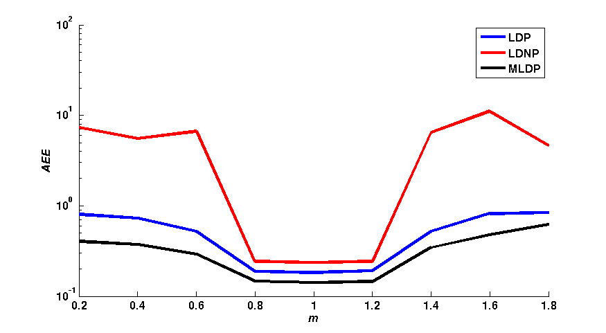
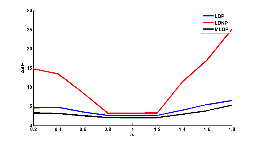
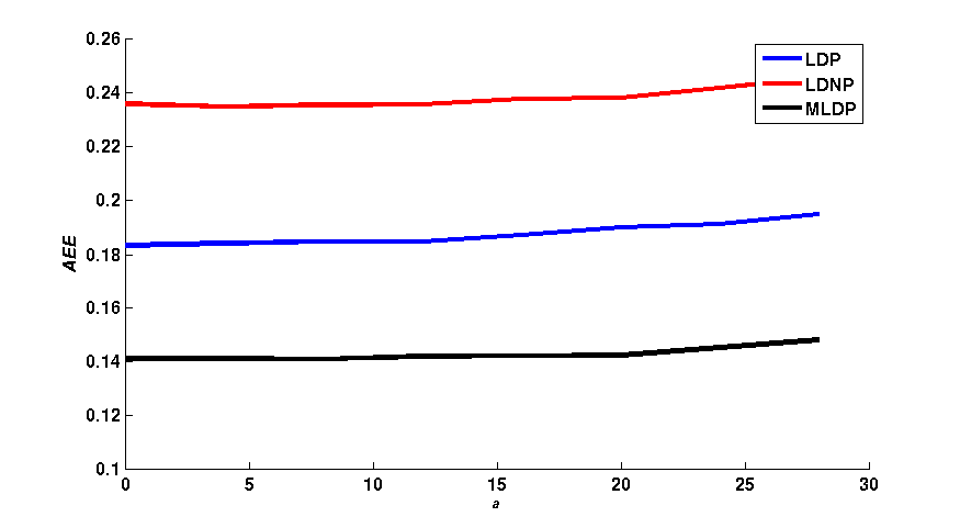
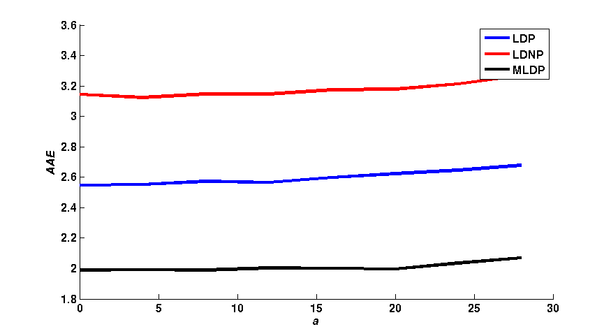
Figure 1 shows a qualitative comparison of the average end-point error (AEE) and the average angular error (AAE) between the flow fields obtained with LDP,
LDNP and MLDP, in a 3 x 3 neighborhood. The effects of different values of m, a and γ have individually been assessed. As shown in figure 1,
the LDNP is robust against small changes of m, a and γ. In turn, LDP and MLDP increase the robustness against both small and large changes of m and γ.
In turn, MLDP yields the smallest AEE and AAE with the change a in turn the LDNP yields the worst values for both AEE and AAE among them.\\
 |
 |
| (a) |
(b) |
 |
 |
| (c) AE = 0.1595 |
(d) AE = 0.0184 |
 |
 |
| (e) AE = 0.0146 |
(f) AE = 0.0452 |
| Fig. 1: (column 1) AEE and (column 2) AAE for LDP, LDNP and MLDP for changing of γ, m and a respectively. |
Weighted Non-Local Term
The effect of the weighted non-local term on the final proposed algorithm has been evaluated.
The AEE and the percentage of the bad pixels (BP) of the obtained flow fields with 8 KITTI
training sequences are calculated for the proposed optical flow technique TV-L1 based on the three descriptors
(LDP, LDNP and MLDP) with and without the weighted non-local term and are shown in table 1. As shown, the values of both AEE and BP for the proposed algorithm are
reduced due to the detected accurate borders after using the weighted non-local term. In addtion, the use of weighted non-local term yields more accurate flow fields.
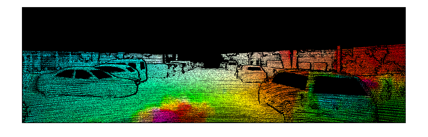
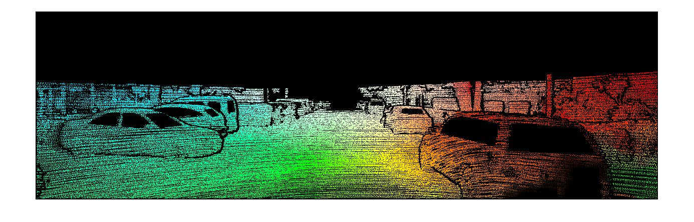
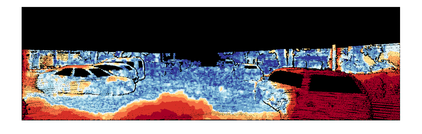
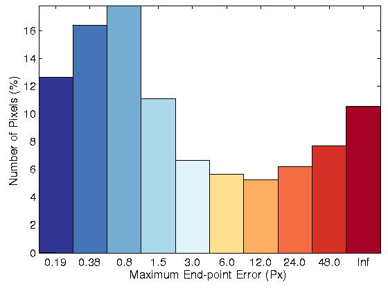
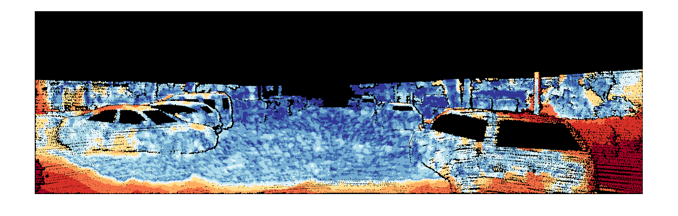
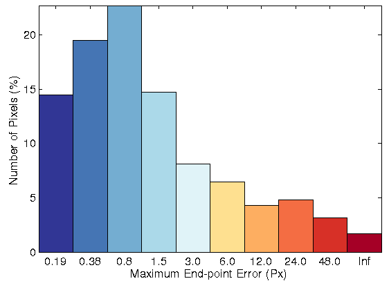
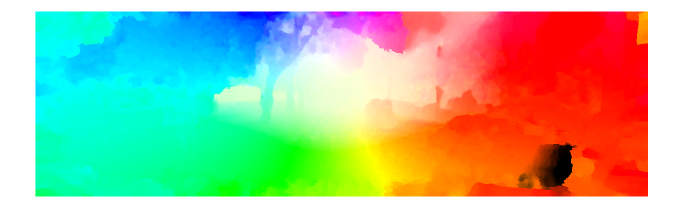
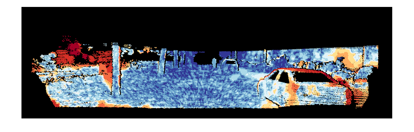
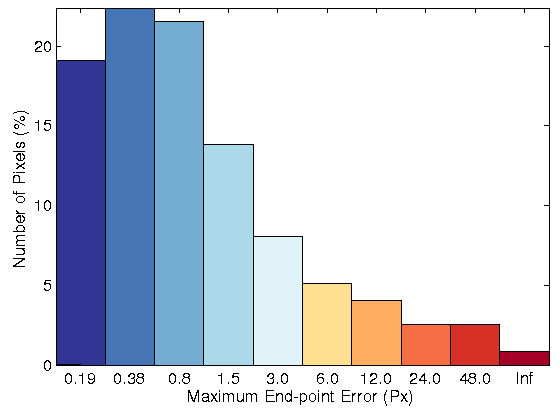
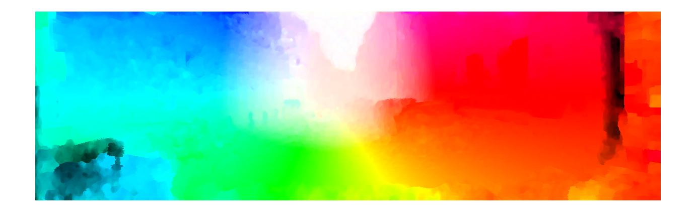
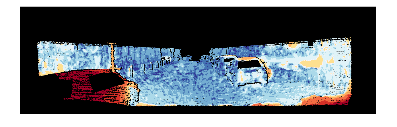
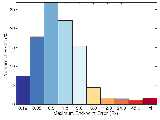
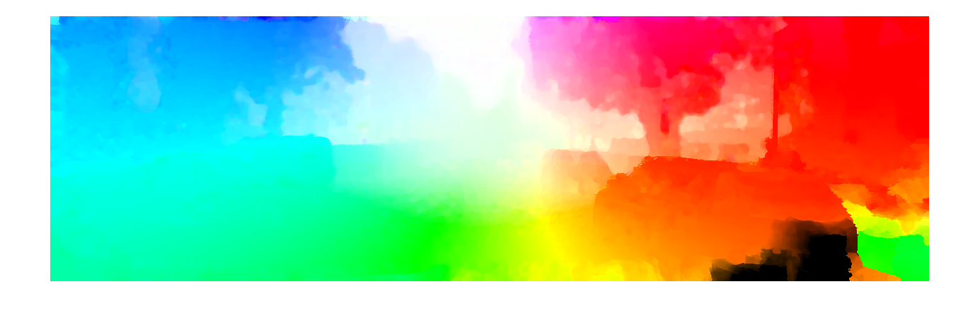
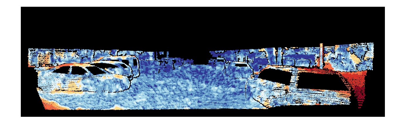
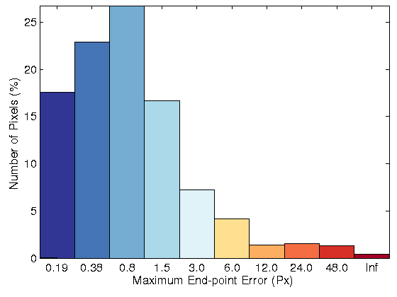
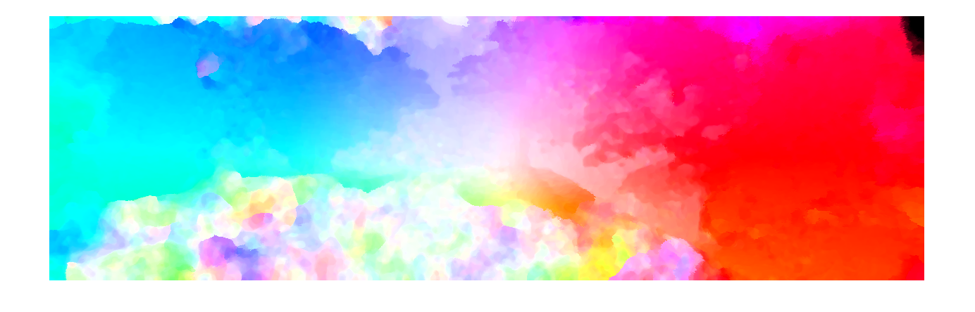
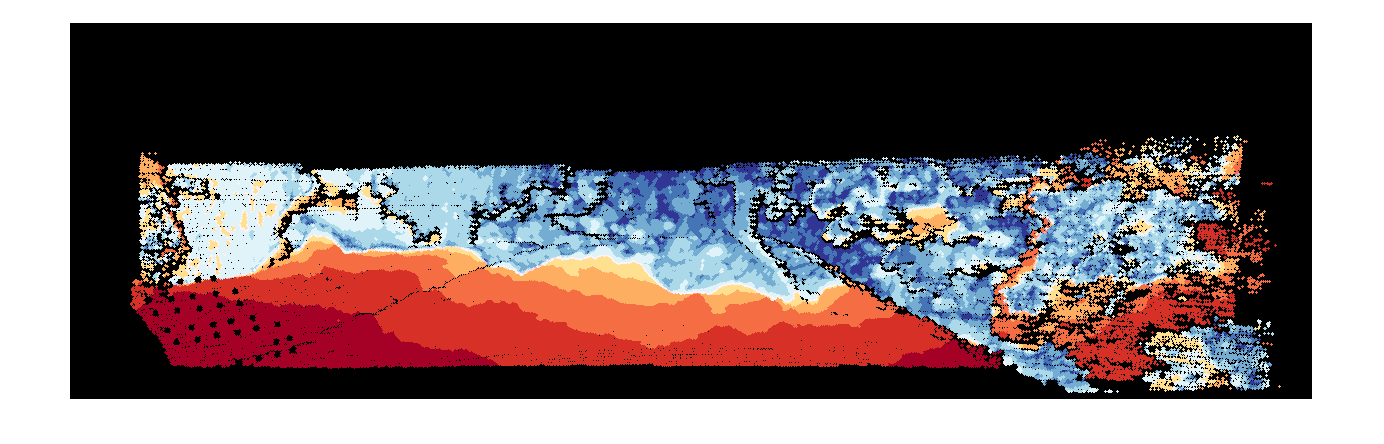
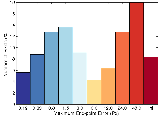
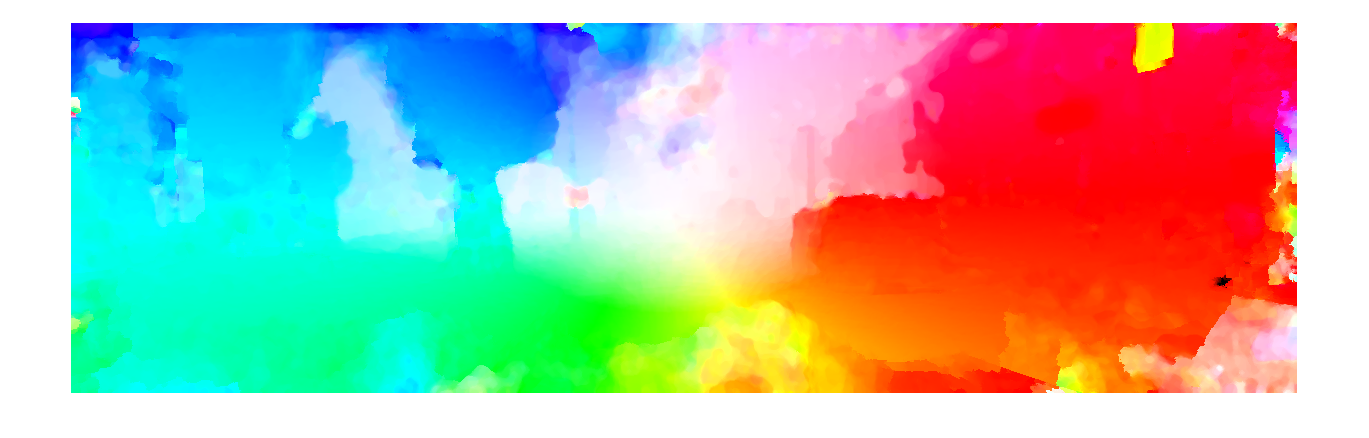
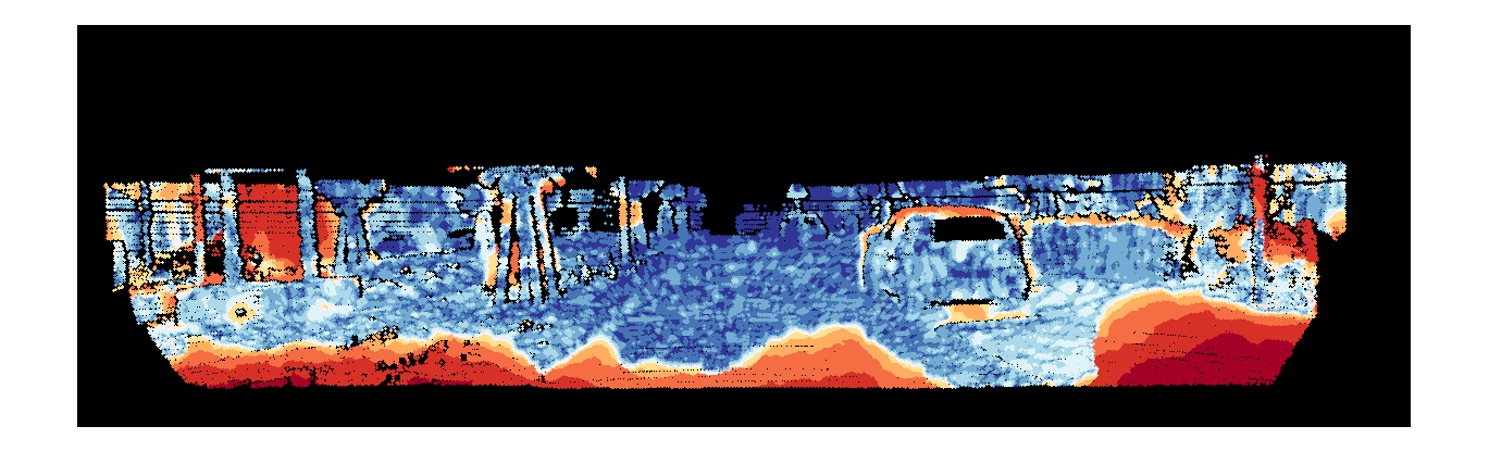
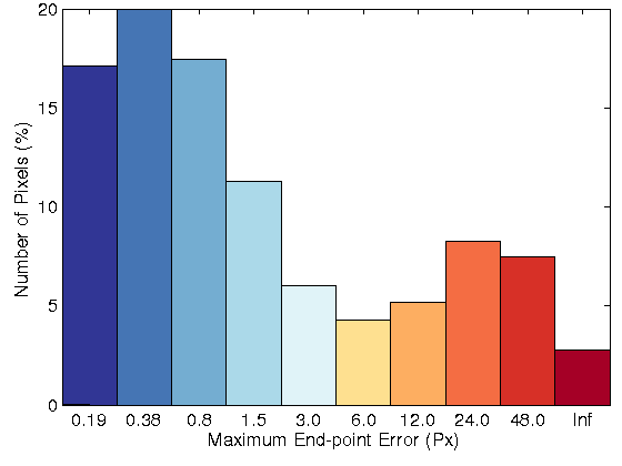
In figure 2, the color flow field, the error image and the histogram of error with and without the non-local term has been visualized. Among LDP, LDNP and MLDP,
the proposed algorithm with an weighted non-local term based on MLDP as data term leads to the best accurate flow fields.
 |
 |
 |
  |
  |
|
|
| Fig. 2: Optical flow model for, Row 1: Original image for sequence 44 of KITTI datasets.
Row 2: Resulting flow field without NL term, Row 3: Resulting flow field with NL term, Row 4: Error image and error histogram without NL, Row 4:
Error image and error histogram with NL term. |
| Sequence | TV-L1 | TV-L1 with Non-Local term |
| | MLDP | LDNP | LDP | MLDP | LDNP | LDP |
| 11 | 35.49%(15.77) | 40.21%(11.41) | 48.26%(26.26) | 29.67% (7.37) | 38.01%(11.14) | 46.19%(16.78) |
| 15 | 26.55%(13.21) | 28.69%(7.74) | 38.27%(18.65) | 23.85% (8.31) | 26.47%(10.64) | 25.58%(7.24) |
| 44 | 35.46%(14.70) | 36.31%(11.27) | 41.11%(16.76) | 20.42% (4.54) | 33.15%(12.00) | 38.27%(11.72) |
| 74 | 61.41%(24.41) | 63.74%(23.68) | 66.73%(24.15) | 56.01% (20.48) | 60.50%(21.49) | 64.36%(26.59) |
| 117 | 31.58%(15.22) | 31.73%(14.88) | 31.91%(15.53) | 18.67% (9.16) | 26.80%(14.89) | 25.27%(7.10) |
| 144 | 47.96%(20.03) | 51.22%(19.27) | 54.81%(18.48) | 41.05% (17.81) | 49.24%(17.09) | 49.55%(18.49) |
| 147 | 18.39%(11.22) | 21.96%(21.65) | 29.22%(19.18) | 11.79% (2.98) | 12.74%(3.90) | 18.76%(13.35) |
| 181 | 59.40%(48.78) | 73.86%(59.62) | 75.83%(58.97) | 58.25% (48.68) | 64.01%(48.94) | 66.07%(53.56) |
KITTI dataset
The proposed variational optical flow method tested upon the widely used KITTI
dataset optical flow. According to the KITTI (July 2013), the results of the proposed model with MLDP
(MLDP_OF)
have been evaluated, and it has been ranked in the 8 position out of 32 current state-of-the-art optical flow algorithms.
The KITTI benchmark considers the bad flow vectors at all pixels that are above a spatial distance of 3 pixels from the ground truth. (MLDP_OF)
has average of 8.90% bad pixels, in turn the baseline methods [7] and [3] have 30.75% and 24.64%, respectively.
| Rank |
Method |
Out-Noc |
Out-All |
Avg-Noc |
Avg-All |
| 1 |
PR-Sf+E |
4.08 % |
7.79 % |
0.9 px |
1.7 px |
| 2 |
PCBP-Flow |
4.08 % |
8.70 % |
0.9 px |
2.2 px |
| 3 |
MotionSLIC |
4.36 % |
10.91 % |
1.0 px |
2.7 px |
| 4 |
PR-Sceneflow |
4.48 % |
8.98 % |
1.3 px |
3.3 px |
| 5 |
TGV2ADCSIFT |
6.55 % |
15.35 % |
1.6 px |
4.5 px |
| 6 |
Data-Flow |
8.22 % |
15.78 % |
2.3 px |
5.7 px |
| 7 |
TVL1-HOG |
8.31 % |
19.21 % |
2.0 px |
6.1 px |
| 8 |
MLDP-OF |
8.91 % |
18.95 % |
2.5 px |
6.7 px |
| 9 |
CRTflow |
9.71 % |
18.88 % |
2.7 px |
6.5 px |
| 10 |
C++ |
10.16 % |
20.29 % |
2.6 px |
7.1 px |
Real illumination and large displacement test
Furthermore, the proposed variational optical flow method based on the MLDP
descriptor is evaluated with eight real image sequences that include illumination
changes and large displacements, as well as low-textured areas, reflections and
specularities. Table 1 shows the AEE and bad pixels corresponding to four se-
quences with illumination changes and large displacements calculated for the
methods proposed in [1] , [2] , [3] ,
[4] , and [5] , in addition to the proposed
method based on MLDP, the census transform and the gradient constancy.
In another experiment, the estimated flow fields with MLDP (3 × 3 and 5 × 5)
have visually been compared with the proposed optical flow method by using
the data term based on the brightness constancy assumption, as well as the
one based on the census transform. Figure 3 shows the estimated flow field for
sequence 15, which includes illumination changes, as well as the error images
and the error histograms. In addition, figure 4 shows the same information for
sequence 181, which includes large displacements. Among the evaluated approaches, the optical flow model based on MLDP
yields the most accurate flow fields with respect to the state-of-the-art methods
for real images of KITTI datasets that include both illumination changes and
large displacements.
Table 1: Percentage of bad pixels and AEE for the state-of-the-art methods
and the proposed method with four sequences from KITTI datasets: sequences
11, 15, 44 and 74, which include illumination changes with the occluded points
ground truth.
| Method |
Seq 44 |
Seq 11 |
Seq 15 |
Seq 74 |
Average |
| MLDP |
20.42% (4.54) |
29.67% (7.37) |
23.85% (8.31) |
56.01% (20.48) |
32.49% |
| Gradient Constancy |
29.25% (9.54) |
35.72%(10.91) |
26.41% (8.47) |
59.20% (23.07) |
37.64% |
| OFH 2011 [5] |
23.22% (5.11) |
37.26% (12.47) |
32.20% (9.06) |
62.90% (24.00) |
38.89% |
| Census(5 x 5) |
35.23% (12.74) |
33.93% (9.75) |
29.04% (8.70) |
57.57% (20.80) |
38.94% |
| Census(3 x 3) |
29.55% (10.22) |
37.54% (11.14) |
33.74% (9.11) |
57.43% (20.53) |
39.56% |
| SRB [3] |
26.58%(4.67) |
40.61% (13.76) |
32.85% (9.72) |
62.94% (24.27) |
40.74% |
| SRBF [3] |
31.83% (5.62) |
40.34% (13.96) |
35.13% (12.17) |
64.89% (24.64) |
43.05% |
| BW [1] |
32.44% (5.19) |
33.95% (8.50) |
47.70% (12.40) |
71.44% (25.15) |
46.38% |
| HS [2] |
42.96% (6.77) |
38.84% (10.72) |
58.08% (12.89) |
82.14% (28.75) |
55.50% |
| WPB [4] |
49.09% (9.20) |
49.99% (28.35) |
67.28% (28.36) |
88.67% (30.68) |
63.76% |
Table 2: Percentage of bad pixels and AEE for the state-of-the-art methods and
the proposed method with four sequences from KITTI datasets: sequences 11,
15, 44 and 74, which include illumination changes with the non-occluded points
ground truth.
| Method |
Seq 44 |
Seq 11 |
Seq 15 |
Seq 74 |
Average |
| MLDP |
8.88% (1.85) |
15.09% (2.87) |
10.22% (2.72) |
49.87% (14.85) |
21.02% |
| Gradient Constancy |
16.78% (4.95) |
19.43%(4.01) |
11.97% (3.52) |
53.13% (16.38) |
25.33% |
| Census(5 x 5) |
24.30% (7.96) |
19.83% (5.06) |
15.03% (3.41) |
51.10%(15.14) |
27.57% |
| OFH [5] |
11.17% (2.44) |
24.32% (6.48) |
18.34% (3.63) |
57.40% (17.25) |
27.81% |
| SRB [3] |
14.66% (2.44) |
27.83% (6.43) |
18.93% (4.05) ) |
57.36% (17.36) |
29.69% |
| Census(3 x 3) |
18.26% (6.30) |
24.05% (7.28) |
20.30% (3.95) |
57.43%(17.53) |
30.01% |
| SRBF [3] |
20.98% (3.29) |
27.78% (6.73) |
21.66% (4.53) |
59.56% (17.52) |
32.49% |
| BW [1] |
22.38% (3.16) |
20.54% (3.62) |
36.85% (6.67) |
67.22% (18.49) |
36.75% |
| HS [2] |
34.18% (4.61) |
25.98% (6.79) |
49.57% (7.95) |
79.57% (21.55) |
47.32% |
| WPB [4] |
40.85% (5.88) |
39.25% (18.75) |
60.50% (17.63) |
87.02% (24.09) |
56.90% |
Sequence 11
 |
 |
| (a) |
(b) |
 |
 |
 |
Brightness Constrain |
 |
 |
 |
Census 3x3 |
 |
 |
 |
Census 5x5 |
 |
 |
 |
MLDP |
| Fig. 1: (row 1) Two original images for sequence 15 of KITTI datasets. Resulting flow field, error image and error histogram for the proposed optical flow model
with: (row 2) brightness constancy, (row 3) 3 × 3 census transform, (row 4) 5 × 5 census transform, and (row 5) MLDP |
Sequence 15
 |
 |
| (a) |
(b) |
 |
 |
 |
Brightness Constrain |
 |
 |
 |
Census 3x3 |
 |
 |
 |
Census 5x5 |
 |
 |
 |
MLDP |
| Fig. 2: (row 1) Two original images for sequence 15 of KITTI datasets. Resulting flow field, error image and error histogram for the proposed optical flow model
with: (row 2) brightness constancy, (row 3) 3 × 3 census transform, (row 4) 5 × 5 census transform, and (row 5) MLDP |
Sequence 44
 |
 |
| (a) |
(b) |
 |
 |
 |
Brightness Constrain |
 |
 |
 |
Census 3x3 |
 |
 |
 |
Census 5x5 |
 |
 |
 |
MLDP |
| Fig. 3: (row 1) Two original images for sequence 15 of KITTI datasets. Resulting flow field, error image and error histogram for the proposed optical flow model
with: (row 2) brightness constancy, (row 3) 3 × 3 census transform, (row 4) 5 × 5 census transform, and (row 5) MLDP |
Sequence 74
 |
 |
| (a) |
(b) |
 |
 |
 |
Brightness Constrain |
 |
 |
 |
Census 3x3 |
 |
 |
 |
Census 5x5 |
 |
 |
 |
MLDP |
| Fig. 4: (row 1) Two original images for sequence 15 of KITTI datasets. Resulting flow field, error image and error histogram for the proposed optical flow model
with: (row 2) brightness constancy, (row 3) 3 × 3 census transform, (row 4) 5 × 5 census transform, and (row 5) MLDP |
Table 3: Percentage of bad pixels and AEE for the state-of-the-art methods and
the proposed method with four sequences from KITTI datasets: sequences 117,
144, 147 and 181, which include large displacement with the occluded points
ground truth.
| Method |
Seq 147 |
Seq 117 |
Seq 144 |
Seq 181 |
Average |
| MLDP > |
11.79% (2.98) |
21.67% (9.16) |
41.05% (17.81) |
59.40% (48.68) |
33.48% |
| OFH [5] |
15.04% (4.96) |
16.26% (4.33) |
42.04% (15.01) |
63.86% (50.52) |
34.30% |
| Gradient Constancy |
12.28% (3.93) |
17.70% (10.81) |
44.51% (18.67) |
67.63% (58.40) |
35.53% |
| SRB [3] |
14.59% (4.85) |
24.71% (9.74) |
50.67% (19.03) |
67.11% (47.70) |
39.27% |
| SRBF [3] |
14.79% (5.17) |
24.41% (9.92) |
50.66% (19.34) |
68.41% (48.81) |
39.57% |
| BW [1] |
16.98% (5.17) |
28.80% (7.86) |
46.98% (16.85) |
69.04% (45.27) |
40.45% |
| Census(5 x 5) |
13.98% (3.41) |
27.33% (15.23) |
47.68% (16.75) |
73.85% (58.59) |
40.71% |
| Census(3 x 3) |
14.76% (3.54) |
28.80% (15.20) |
48.97% (16.83) |
73.63% (58.58) |
41.54% |
| HS [2] |
24.84% (6.61) |
43.24% (15.32) |
51.89% (14.81) |
74.11% (49.28) |
48.52% |
| WPB [4] |
32.72% (8.10) |
46.80% (13.67) |
52.25% (17.94) |
76.00% (50.18) |
51.94% |
Table 4: Percentage of bad pixels and AEE for the state-of-the-art methods
and the proposed method with four sequences from KITTI datasets: sequences
117, 144, 147 and 181, which include large displacement with the non-occluded
points ground truth.
| Method |
Seq 147 |
Seq 117 |
Seq 144 |
Seq 181 |
Average |
| MLDP > |
4.66% (1.05) |
13.80% (4.19) |
28.02% (6.93) |
46.81% (21.03) |
23.32% |
| OFH [5] |
8.03% (1.98) |
9.09% (2.17) |
29.62% (6.77) |
52.32% (23.46) |
24.76% |
| Gradient Constancy |
7.13% (1.25) |
9.70% (4.42) |
32.25% (8.26) |
57.21% (29.92) |
26.57% |
| SRB [3] |
7.55% (1.74) |
18.11% (5.28) |
39.55% (9.33) |
56.51% (22.88) |
30.43% |
| SRBF [3] |
7.69% (1.97) |
17.95% (5.29) |
39.64% (9.59) ) |
58.25% (23.78) |
30.88% |
| BW [1] |
10.07% (2.20) |
22.25% (4.23) |
35.01% (8.17) |
59.05% (22.58) |
31.60% |
| Census(5 x 5) |
6.78% (0.95) |
20.52% (9.82) |
36.29% (7.71) |
65.55% (31.26) |
32.29% |
| Census(3 x 3) |
6.63% (1.00) |
21.85% (9.59) |
37.49% (8.43) |
65.29% (31.92) |
32.82% |
| HS [2] |
18.52% (3.38) |
37.82% (9.77) |
41.30% (7.32) |
65.77% (23.40) |
40.85% |
| WPB [4] |
25.92% (4.43) |
41.23% (9.18) |
41.53% (8.94) |
68.27% (25.96) |
44.24% |
Sequence 144
 |
 |
| (a) |
(b) |
 |
 |
 |
Brightness Constrain |
 |
 |
 |
Census 3x3 |
 |
 |
 |
Census 5x5 |
 |
 |
 |
MLDP |
| Fig. 5: (row 1) Two original images for sequence 15 of KITTI datasets. Resulting flow field, error image and error histogram for the proposed optical flow model
with: (row 2) brightness constancy, (row 3) 3 × 3 census transform, (row 4) 5 × 5 census transform, and (row 5) MLDP |
Sequence 147
 |
 |
| (a) |
(b) |
 |
 |
 |
Brightness Constrain |
 |
 |
 |
Census 3x3 |
 |
 |
 |
Census 5x5 |
 |
 |
 |
MLDP |
| Fig. 6: (row 1) Two original images for sequence 15 of KITTI datasets. Resulting flow field, error image and error histogram for the proposed optical flow model
with: (row 2) brightness constancy, (row 3) 3 × 3 census transform, (row 4) 5 × 5 census transform, and (row 5) MLDP |
Sequence 117
 |
 |
| (a) |
(b) |
 |
 |
 |
Brightness Constrain |
 |
 |
 |
Census 3x3 |
 |
 |
 |
Census 5x5 |
 |
 |
 |
MLDP |
| Fig. 7: (row 1) Two original images for sequence 15 of KITTI datasets. Resulting flow field, error image and error histogram for the proposed optical flow model
with: (row 2) brightness constancy, (row 3) 3 × 3 census transform, (row 4) 5 × 5 census transform, and (row 5) MLDP |
Sequence 181
 |
 |
| (a) |
(b) |
 |
 |
 |
Brightness Constrain |
 |
 |
 |
Census 3x3 |
 |
 |
 |
Census 5x5 |
 |
 |
 |
HOG 3x3 |
 |
 |
 |
MLDP |
| Fig. 8: (row 1) Two original images for sequence 15 of KITTI datasets. Resulting flow field, error image and error histogram for the proposed optical flow model
with: (row 2) brightness constancy, (row 3) 3 × 3 census transform, (row 4) 5 × 5 census transform, and (row 5) MLDP |
References
| 1. |
A. Bruhn and J. Weickert. Towards ultimate motion estimation: Combining highest accuracy with real-time performance. In ICCV, pages 749-755, 2005. |
| 2. |
B. Horn and B. Schunk. Determining optical flow. In Artificial Intelligence, vol. 17, pages 185-203, 1981. |
| 3. |
D. Sun, S. Roth, and M.J. Black. Secrets of optical flow estimation and their principles. In CVPR, pages 24322439. IEEE, 2010. |
| 4. |
M. Werlberger, T. Pock, and H. Bischof. Motion estimation with non-local total variation regularization. In CVPR, pages 2464-2471.IEEE, 2010. |
| 5. |
H. Zimmer, A. Bruhn, and J. Weickert. Optic flow in harmony. In IJCV, vol. 93(3): pages 368-388, 2011. |
| 6. |
Rudin, L.I., Osher, S.J., Fatemi, E.: Nonlinear total variation based noise removal algorithms. In Physica D, vol. 60, pages 259-268, 1992 |
| 7. |
C. Zach, T. Pock, H. Bischof, A duality based approach for realtime tv- l1 optical flow. In DAGM. pages 214-223, 2007 |
| 8. |
M. Mohamed, H. Rashwan, B. Mertsching, M. Garcia, and D. Puig.
Illumination-Robust Optical Flow Using Local Directional Pattern.
In: IEEE Transactions on Circuits and Systems for Video Technology, 2014. |
Contact
Do you have any questions or comments? Please contact:
|